Article

GIS and Machine Learning Models Target Dynamic Settlement Patterns and Their Driving Mechanisms from the Neolithic to Bronze Age in the Northeastern Tibetan Plateau

1
Ministry of Education Key Laboratory of Western China’s Environmental System, College of Earth and Environmental Sciences, Lanzhou University, Lanzhou 730000, China
2
School of Mathematics and Statistics, Lanzhou University, Lanzhou 730000, China
3
School of Geographical Sciences and Tourism, Zhaotong University, Zhaotong 657000, China
*
Author to whom correspondence should be addressed.
Submission received: 30 March 2024 / Revised: 11 April 2024 / Accepted: 15 April 2024 / Published: 19 April 2024
(This article belongs to the Section Environmental Remote Sensing)

Abstract

:
Traditional GIS-based statistical models are intended to extrapolate patterns of settlements and their interactions with the environment. They contribute significantly to our knowledge of past human–land relationships. Yet, these models are often criticized for their empiricism, lopsided specific factors, and for overlooking the synergy between variables. Though largely untested, machine learning and artificial intelligence methods have the potential to overcome these shortcomings comprehensively and objectively. The northeastern Tibetan Plateau (NETP) is characterized by diverse environments and significant changes to the social system from the Neolithic to Bronze Age. In this study, this area serves as a representative case for assessing the complex relationships between settlement locations and geographic environments, taking full advantages of these new models. We have explored a novel modeling case by employing GIS and random forests to consider multiple factors, including terrain, vegetation, soil, climate, hydrology, and land suitability, to construct classification models identifying environmental variation across different cultural periods. The model exhibited strong performance and a high archaeological prediction value. Potential living maps were generated for each cultural stage, revealing distinct environmental selection strategies from the Neolithic to Bronze Age. The key environmental parameters of elevation, climate, soil erosion, and cultivated land suitability were calculated with high weights, influencing human environmental decisions synergistically. Furthermore, we conducted a quantitative analysis of temporal dynamics in climate and subsistence to understand driving mechanisms behind environmental strategies. These findings suggest that past human environmental strategies were based on the comprehensive consideration of various factors, coupled with their social economic scenario. Such subsistence-oriented activities supported human beings in overcoming elevation limitation, and thus allowed them to inhabit wider pastoral areas. This study showcases the potential of machine learning in predicting archaeological probabilities and in interpreting the environmental influence on settlement patterns.

1. Introduction

The location of settlements is not random but reflects human sensibility, aligning with landscape attraction and socioeconomic structure [1,2,3,4]. Thus, exploring settlement patterns and uncovering the mechanisms of human environmental strategies is crucial for interpreting past human–land relationships. Owing to the accumulation of archaeological data as well as the advancements in computer science over the past few decades, using GIS technology for digital data analysis has yielded significant achievements for settlement and landscape archaeology [5,6,7]. Archaeological predictive modeling (APM) is a powerful tool for explaining settlement patterns and environmental causation, and it can be effectively used as a guide for heritage surveys to assess the likelihood of land to contain new archaeological sites [8,9,10]. More recently, innovative approaches, such as machine learning (ML) and artificial intelligence (AI) approaches, have the potential to enhance APM performance and to unearth more valuable archaeological insights [11,12].
APM has been developed over 40 years and primarily utilizes binary classification methods [13,14]. It typically involves dependent factors regarding known sites and random points, and independent variables encompassing various environmental factors. The classical statistical method of logistic regression has been widely used for predictive modeling, but it is prone to underfitting and low accuracy [2,7,10,11,15]. Newer models like maximum entropy, weight-of-evidence, and deletion/substitution/addition have also been explored to improve performance and archaeological interpretation [1,3,4,6,16]. However, these models perform weakly when handling some complex relationships. ML presents an opportunity to enhance predictive accuracy and to provide richer archaeological interpretability. For instance, Liu simulated the prehistoric agricultural dispersal routes based on several ML methods in the Tibetan Plateau (TP) and demonstrated that random forests (RFs) achieved the highest classification accuracy and that logistic regression yielded the lowest [12]. Guo suggested that gradient ascent algorithms can greatly improve the accuracy of logistic regression in AMP [11]. Some similar cases in geological hazard evaluation have also shown that tree-based models like RFs and XGBoost perform well in accuracy, robustness, and generalization ability [17,18,19]. Furthermore, deep learning technology has rapidly developed in GIS and RS fields to the point that neural networks can better explain some uncertain “quantum relationships” [20,21,22,23]. The application of ML in settlement archaeology remains scarce, however. Various supervised classification, unsupervised clustering, and dimensionality reduction technologies can be effectively exploited in ML to handle and interpret some complex human–environment interaction processes with new perspectives.
The northeastern Tibetan Plateau (NETP) stands out as a crucial zone for examining complex human–environmental interactions, particularly during the period from the Neolithic to Bronze Age, as agricultural economies developed and when year-round sedentary lifestyles dominated [24,25,26,27]. This region can serve as an exceptional case study for the use of ML due to the complex geographic landforms and the course of culture. Chen et al. proposed a stepwise pattern of human occupation on the TP using a systematic AMS 14C chronology and archaeological survey [24]. Around 5200 BP, millet farmers began farming intensively, inhabiting low-elevation regions (<2500 m a.s.l.) of the NETP. Until 3600 BP, the introduction and growth of trans-continental economies of wheat–barley agriculture and cattle–sheep pastoral activities acted as a buffer against climate change and facilitated sustained human occupation in high-altitude regions (>2500 m a.s.l.) of the TP [24]. This pattern has been further corroborated and enriched by subsequent archaeological and genetic discoveries [28,29,30]. Although this occupation timeline has been basically outlined, the process details and the variation in human behavior across cultures remain unclear. Furthermore, our existing knowledge has emphasized the unique influence of elevation in the TP, but other factors crucial for survival, particularly the coexistence of agricultural and pastoral economies in the NETP, have been insufficiently considered. GIS combined with machine learning techniques can provide a new method for interpreting these issues in-depth.
The presence of archaeological settlements indicates sustained human activity in the past and calls for an in-depth GIS analysis through the integration of digital geographic data [31,32]. Previous discussions, which primarily relied on GIS visualization and spatial analysis, have demonstrated that social subsistence in the NETP heavily influenced settlement distribution patterns during different cultural periods [33,34,35]. On the other hand, trans-continental cultural exchange and climate fluctuation served as underlying factors in shaping societal patterns [34,35,36]. Many studies have explored these perspectives and proposed more factors influencing human activities, including hydrological, topographical, and vegetation factors. For example, d’Alpoim Guedes emphasized that the effective accumulated temperature plays a pivotal role in agricultural cropping [25,37]. Hou and Ma’s studies proposed that the distance to a river also influences agricultural settlements [35,38]. Liu demonstrated that elevation, vegetation, river distance, slope, and surface fluctuation collectively influenced ancient migration patterns and settlements in the prehistoric TP [12]. Chen proposed that herder mobility followed an ecological-oriented strategy from the Bronze to the Iron Age in the TP [39]. Moreover, some studies intending to reconstruct ancient traffic routes of the TP have tried to integrate various factors to simulate a moving cost surface [27,40,41,42]. However, these studies either only considered the influence of single factors, one at a time, or determined the weights of various geographic factors through empirical assessment using tools such as the Analytical Hierarchy Process [43]. APM based on available data appears to be relatively objective and comprehensive in evaluating environmental rules on settlement selection [4]. Using ML models offers the great advantages of incorporating a wider range of potential factors to enhance accuracy and of implementing optimal filtering objectively [44].
Our present study focused on dynamic environmental strategies during different cultural periods in crucial areas of the NETP. To achieve this, we undertook a methodological exploration using supervised classification tree and random forest algorithms to construct classifiers for archaeological potential prediction and to interpret human environmental strategies. Additional environmental data that may have potentially influenced settlements patterns were involved to increase model reliability. Unsupervised Self-Organizing Map (SOM) techniques were also applied to visually depict the adaptation process. Furthermore, the driving mechanism behind the human occupation of high-altitude environments of the NETP was quantitatively analyzed by investigating climate and socioeconomic changes during the period from the Neolithic to the Bronze Age.

2. Materials and Methods
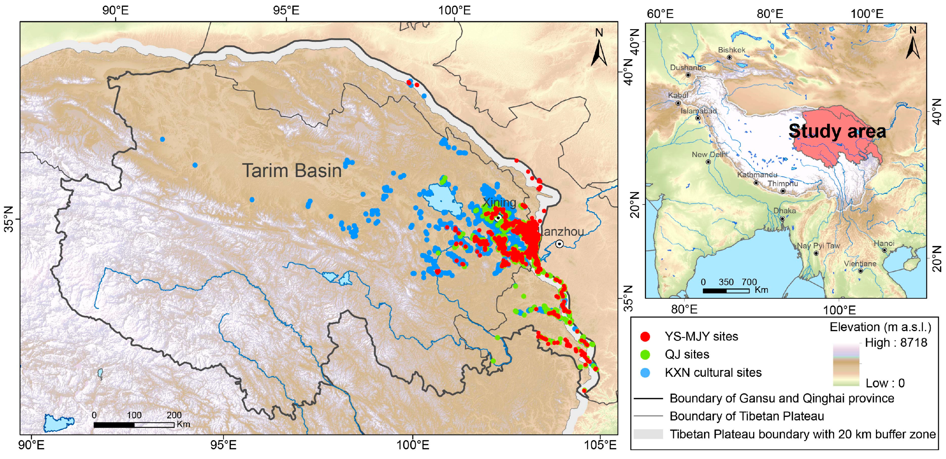
2.1. Study Area

The NETP is defined in this study as the region where the TP intersects Gansu and Qinghai provinces (Figure 1). To account for the influence of adjacent areas, a 20 km buffer zone was added along the border of the TP. The natural environments in the NETP are diverse, with a complex topography and significant variations in regional landscapes that are heavily influenced by elevation [45,46]. The elevation in the NETP ranges between 928 and 6818 m, accompanied by a variety of landform types including plains, basins, hills, and mountains [47]. Based on data from 62 meteorological stations in the NETP, the annual temperature varies greatly (from −5.1 to 15.1 °C), with an average temperature of 4.2 °C. The average annual precipitation ranges from 15 to over 700 mm (http://data.cma.cn, accessed on 20 March 2024). The area sits in a typical semi-arid and semi-humid junction. Being situated in a marginal monsoon region, the climate, vegetation, and other landscape attributes of the TP are sensitive to global environmental change [48]. Furthermore, being centrally positioned in the eastern segment of the Silk Road, the NETP serves as a pivotal hub for continental cultural exchange and agricultural dispersal, with many exotic elements having emerged early in this region early on [48,49,50].

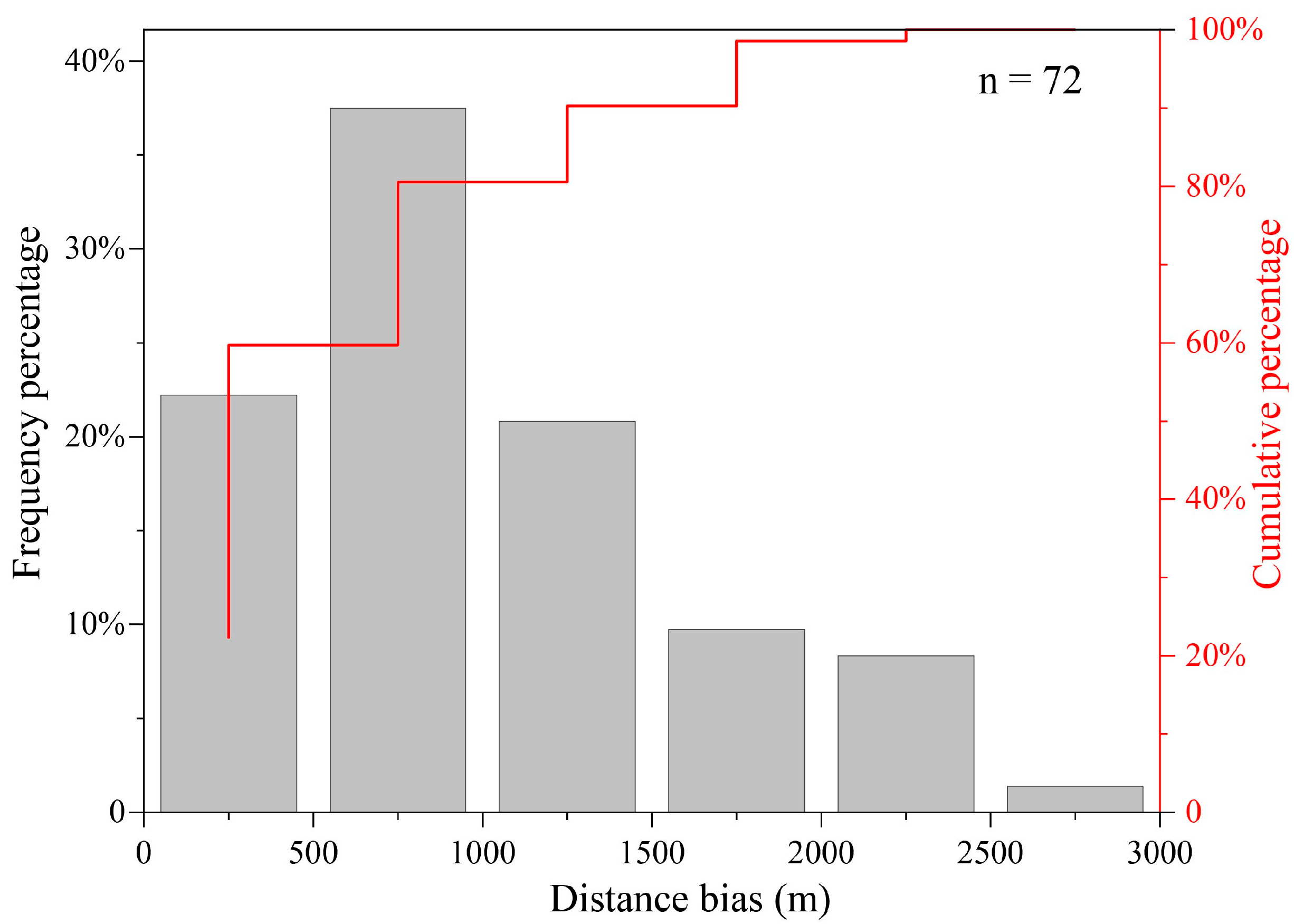
2.2. Archaeological Context and Data

By reviewing the archaeological cultural lineage and features from the Neolithic to Bronze Age in the NETP, we have identified three major cultural periods: the Yangshao-Majiayao (YS-MJY) period, the Qijia (QJ) period, and the Kayue-Xindian-Nuomuhun (KXN) period [51]. The YS-MJY period (5500–4000 BP) in the Neolithic era encompassed major cultures such as the Later Yangshao culture (5500–5000 BP), the Majiayao culture (5300–3900 BP), and the Zongri culture (5600–4000 BP) [51,52]. Among these, the Majiayao culture, which derived from the Yangshao culture, was the most widely distributed in the NETP. The YS-MJY period contains three phases: the Majiayao phase (5300–4600 BP), the Banshan phase (4600–4300 BP) and the Machang phase (4300–3900 BP) [28,53]. The Zongri culture (5600–4000 BP) was an aboriginal culture that coexisted and interacted with Mjiayao culture and was predominantly distributed in the higher altitudes of the Gonghe and Guide basins [29,51]. The QJ culture (4300–3600 BP) was a transitional culture spanning the Neolithic to Bronze Age [54,55]. In the early period of QJ culture (4300–4000 BP), no bronze artifacts were found, while in the middle and later periods (4000–3600 BP), bronze artifacts were discovered in many sites, which led to the latter period being classified as the beginning of the Bronze Age [56,57,58]. However, the cultural features and characteristics of QJ culture were consistent throughout the early, middle, and late periods [57,59]. After 3600 BP, the uniform culture separated into multiple cultures. The NETP mainly included the Kayue culture (3600–2100 BP), the Xindian culture (3600–2500 BP), and the Nuomuhong culture (3400–2500 BP) [60,61]. These cultures are typical of the Bronze Age cultures and influenced by QJ culture [58,62,63].
The data used in this study, which include site locations and cultural attributes from the Neolithic to the Bronze Age, are derived from the Chinese Cultural Relic Atlas, a digital database constructed using map scanning that can be accessed on the internet [64,65,66]. This dataset comprises a total of 3168 records in our study area. Most of these sites represent inhabited sites, and the remaining small parts are burial sites. Here, we unified all of the sites as settlements because both indicate evidence of sustained human activity and can be considered as parts of a ‘settlement’ in a broad sense. Moreover, burials were typically performed close to living areas during the Neolithic to the Bronze Age in the NETP [67,68,69]. The location quality of the data was also evaluated by cross-referencing with the precise locations of known archaeological sites. These known sites were identified using 14C data; these data were also used in the temporal analysis in Section 4.2. In addition, we simulated 1600 random points as non-sites. To ensure the validity of these random points, these non-site points were situated outside a 5 km buffer area surrounding the actual sites because prehistoric human activity was generally concentrated within approximately 5 km of settlements [70]. Using random points as virtual sites is a widely used method that is comparable to the rational selection of an environment by humans [1,2,3,4,5,6,7,8,9,10,11,12,13,14,15,16]. As a result, the dependent variables used for the model include four categories: YS-MJY (n = 766), QJ (n = 733), KXN (n = 1649), and non-sites (n = 1600).

2.3. Environmental Data

We considered six types of geographical and environmental factors, encompassing a total of 16 variables. These factors included terrain, vegetation, hydrology, soil, climate, and agricultural suitability, all of which have the potential to influence human activity. For example, a high elevation site faces low temperature and low oxygen, which influence human physiology and survival [71]. Other terrain factors may impact human mobility costs, light exposure, drainage, air circulation, or disasters [10,40,41]. Vegetation and hydrology play crucial roles in determining the availability of natural resources and water. Soil and climatic conditions heavily influence human agricultural practices. Land suitability is a composite indicator assessing both cultivated land suitability and pastoral land suitability. These two indictors determined farmers’ and herders’ subsistence-oriented activities [39]. Following the method of Yao et al. [72], we classified agricultural and pastural areas into four levels: high, moderate, marginal, and unsuitable. Class thresholds were established using the Jenks class method [73]. For further details, see Supplementary Materials. For the geographic data, most of the preprocessing and data extraction processes were implemented in R, which is available in GitHub. For a comprehensive overview of data sources and processing methods, specific details are shown in Table 1.

2.4. Creating the Models

Through preliminary testing, RFs demonstrated excellent performance in terms of classification accuracy, robustness, and interpretability. Numerous similar studies have also reported these advantages, and the RF model has been widely applied for spatial prediction [12,17,18,79]. In our current study, we constructed a multi-classification RF model to predict cultural potential probabilities in a landscape scale across the entire NETP. An explanatory classification tree was also employed for archaeological interpretation. The modeling process is shown in Figure 2. To comprehensively explore the influence of multiple variables on settlement selection, we employed an unsupervised SOM to further investigate landscape differences from the Neolithic to Bronze Age. The main R packages used are introduced in Table 2.

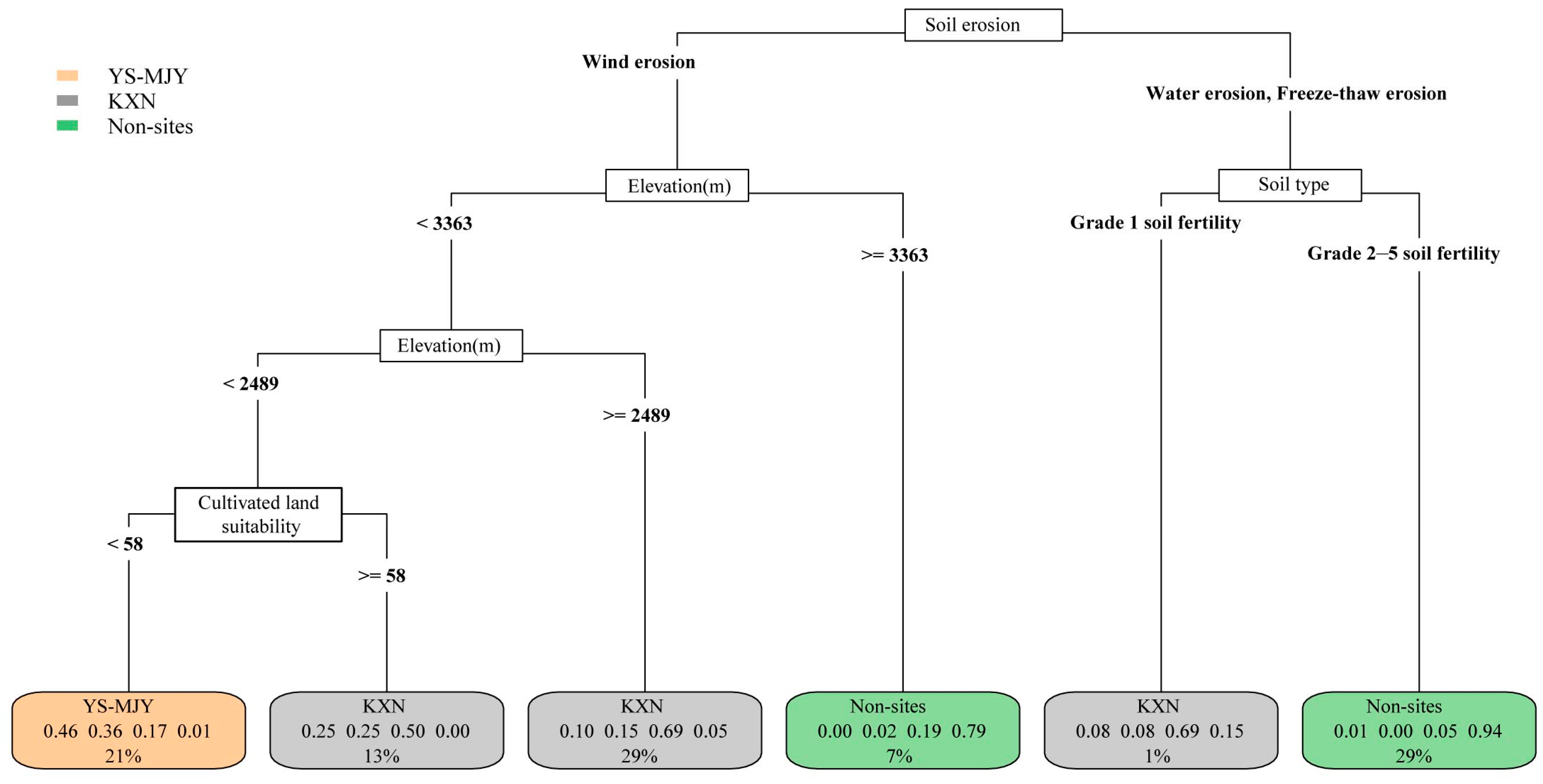
2.4.1. Classification Tree

The classification tree (i.e., decision tree) established a tree-like structure to depict the relationships between features (independent variables) and classification outcomes. The prevalent algorithm for building classification trees is through a binary recursive partitioning (rpart). This algorithm considers all predictor variables and selects those that differentiate between categories effectively [90]. The process involves iteratively splitting the data into partitions and further splitting the data up further on each of the branches until each subset belongs to the same label. The standard techniques for selecting the best features are based on the Gini index gain, which aims to maximize the reduction in impurity. Pruning is often necessary to optimize the tree. Classification trees offer easy interpretability, as they provide straightforward explanations of decision paths. However, they focus on local information, so there is a risk of overfitting. Hence, these trees often serve as relatively weak classifiers [44,91].
G i n i = 1 1 K p X k 2
G i n i   g a i n   =   p a r e n t   n o d e   G i n i     c h i l d   n o d e   G i n i
  • K: Number of classes;
  • Xk: Class k; k = 1, …, K;
  • p(Xk): The classification probability of Xk.

2.4.2. Random Forests

The RF model is a popular ensemble machine learning algorithm making use of the “bagging” strategy and is usually used to boost the performance of decision trees [92]. The core concept involves randomly selecting samples as training datasets to construct decision trees. At each split node of these trees, features are also randomly selected. By repeating those random sampling processes, multiple decision trees are generated. Each decision tree that constitutes the RF model will predict an output result, and ultimately, the voting outcomes of each tree determine the final result. The unsampled data in each tree training process can be used to validate the model, generating “out-of-bag (OOB) errors” to verify the model’s accuracy. The voting results of multiple trees also determine the classification probability. The importance of each variable is determined by calculating the average decrease in Gini impurity across all decision trees in the RF model. In all, the RF model effectively solves the overfitting problem of a decision tree and improves model performance. The model is relatively robust and provides an interpretable variable importance ranking [44]. The RF model has now been widely used in geohazard assessment, paleoenvironment reconstruction, and remote sensing interpretation [12,17,18,79].
Before model training, variable selection and parameter optimization should be carried out to ensure that different algorithms perform classification tasks under the optimal variables and parameters. A feature evaluation strategy employing a filter method was used to exclude factors with a Pearson correlation coefficient greater than 0.8. This helped mitigate the impact of strong multicollinearity on model performance. Parameter optimization was carried out using random search and K-fold cross-validation methods (with K set to 5). In the random search method, hyperparameter values were randomly selected from a predefined range for each iteration. This method did not rely on exhaustive searching through all possible hyperparameter combinations, making it computationally more efficient [44,93]. By randomly sampling from the parameter space, the random search method had the potential to discover optimal or near-optimal hyperparameter configurations [44]. The K-fold cross-validation (CV) method was used to assess the performance of a model and to estimate its generalization error. The dataset was divided into K subsets (or folds), and the model was trained and evaluated K times, each time using a different fold as the validation set with the remaining folds as the training set. The performance accuracy was calculated as the average of the performance scores across all K folds. Combining random search with K-fold CV methods for parameter optimization involved performing random search iterations when evaluating each hyperparameter configuration using the CV method [44,93].

2.4.3. Model Assessment

We used OOB, holdout validation, and K-fold CV methods to examine the RF model classification performance. The OOB error was generated using the RF model. Holdout validation was conducted, with 80% as the training set and 20% as the test set. To avoid statistical coincidence, the K-fold CV method was also applied, as mentioned above. We set K = 10 and repeated the sampling process five times. The model performance was assessed using accuracy, confusion matrix, kappa, and the AUC. The confusion matrix was used to evaluate the performance of a classification model by comparing the model’s predictions against the actual labels. Kappa measures the model’s performance beyond random guessing in a classification task [94]. The AUC, “area under the receiver operating characteristic (ROC) curve”, represented the overall performance of the classification models [95,96]. The ROC curve was the graphical representation of the true positive rate versus the false positive rate at different classification thresholds [95]. In the context of multi-class classification, the AUC is computed by treating each class as the positive class and all others as the negative class, thus resulting in a set of binary classification problems [95]. When the kappa and AUC values are closer to 1, the model performs better [94].
To further verify the model predicting performance, we introduced the Kvamme gain index, which is widely used in APM assessing and focuses on balancing the ratio of true positives to false positives [13,97]. As the gain approaches 1, the predictability of the model increases.
G a i n = 1 p m / p s
  • pm is the ratio of the probability area to the total study area;
  • ps is the ratio of the number of sites in the probability area to the total number of sites.

2.4.4. Self-Organizing Maps

Self-Organizing Maps (SOMs) are unsupervised learning neural networks applied for clustering, mapping, and non-linear dimensionality reduction [98,99,100]. They were inspired by biological models of neural systems from the 1970s [98]. SOMs have two layers: the input layer and the output layer. The input layer represents a high-dimensional dataset, such as the 16-dimensional features used in this study. The SOM (output layer) is typically visualized as a two-dimensional sheet with neurons arranged in a k × l lattice, where each element represents a neuron node. These neural networks employ a competitive learning approach, gradually optimizing the network by competition between neurons or nodes. Hence, high-dimensional data based on similarities within the input dataset can be mapped to nearby nodes in the two-dimensional space.
We assumed an input data of size (M, N) where M is the number of training examples and N is the number of features in each example. The following steps outline the self-organization process in Self-Organizing Maps (SOMs):
Initialization: Create a k × l lattice as a SOM grid. All SOM nodes are arbitrarily positioned to random values, usually using small numbers.
Competition: A random input vector m is selected, and the Euclidean distance between m and each neuron node in the SOM grid is calculated. After calculating the distances, the neuron closest to the input vector m is identified. This neuron is called the Best Matching Unit (BMU) or winner node.
Cooperation: The cooperation phase begins after finding the BMU. In this phase, the BMU’s neighbors are updated. The neighborhood is defined using a neighborhood function h, which quantifies the degree to which a neuron can be considered a neighbor of the winning neuron. The basic principle is that neurons closer to the winning node have a greater updating range, while those further away have a smaller update amplitude. The Gaussian function (Equation (4)) is commonly used to assess the influence of the BMU on the neighboring neurons.
h d i , j = e d 2 ( i , j ) 2 σ 2
  • d(i, j): distance between neighbor j and the winning neuron BMU i.
  • σ: the standard deviation of the Gaussian function.
Adaptation: Here, the weights of all neurons are updated according to the neighborhood function h:
Wj(n + 1) = Wj(n) + αhij (d (m, Wj(n))
  • n represents the nth iteration;
  • m is the select input vector;
  • Wj(n) is the weight of neighbor neuron j at iteration nth;
  • i represents the BMU;
  • α is the learning rate;
  • d is a distance function.
Iteration: after completing one iteration (incrementing the number of iterations n + 1), the SOM returns to the competition step until the set number of iterations is met.
This technology was employed to understand the occupation process at different cultural stages in the NETP. Primary hyperparameters were set as follows: learning rate α from 0.05 to 1, iteration numbers rlen = 5000, size of the grid k × l = 20 × 20, topological structure set to “rectangular”, neighborhood function h set to “gaussian”. SOMs can effectively handle complex data. They are good for visualization and allow people to reduce complex problems with their easy interpretation. Now, SOMs have been successfully used to assess the grade of settlement [101]. But SOMs are not suitable for processing small amounts of data; hence, a typical principal component analysis (PCA) was used as a supplementary method for analyzing small amounts of data in the discussion part [100].

2.4.5. Principal Component Analysis

Principal component analysis (PCA) is a linear dimensionality reduction technique widely applied in exploratory data analysis, visualization, and data preprocessing. It can extract important information and eliminate redundant (intercorrelated) data. The main steps of PCA are as follows: (1) Data standardization. (2) Covariance matrix computation: the covariance matrix of the standardized data is calculated, representing the relationships between different features. (3) Eigenvalue decomposition: the covariance matrix is decomposed into its eigenvectors and eigenvalues. (4) Selection of principal components: the eigenvectors corresponding to the largest eigenvalues are selected as the principal components, determining the directions of maximum variance in the data. (5) Projection: the original data are projected onto the selected principal components to obtain the lower-dimensional representation of the data. (6) Visualization: the top two or three principal components are used to construct 2D or 3D PCA score maps.

3. Results

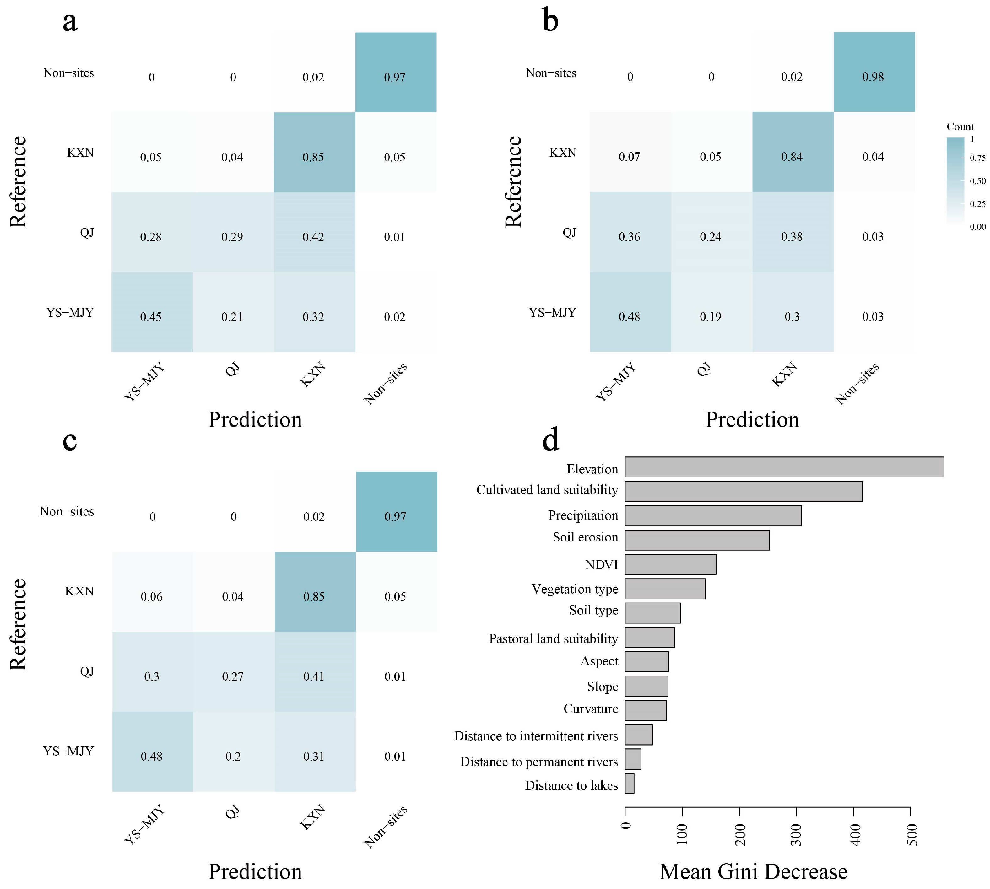
3.1. Data Assessment and Model Optimization

By comparing the locations of 72 known sites with those in the ‘Chinese Cultural Relic Atlas dataset’, we calculated the following positional deviation curves (Figure 3). The results show that ~60% of the site locations have a deviation within 1000 m and ~80% of the site locations have a deviation within 2000 m. This level of error might affect the interpretation of the microtopographic environment to some extent, but it minimally impacts the understanding of the broader, macroscopic distribution patterns. Hence, it was decided to construct a predictive model with a resolution of 1 km to achieve a reliable prediction in landscape scales.
After calculating the Pearson correlation coefficient matrix of variables, we found fluctuations that showed a high correlation with slope and that temperature highly correlated with elevation (Figure S3). We excluded fluctuation and temperature factors in the modeling. The results of the hyperparameter optimization of the RF model indicate that the number of decision trees was set to 926 (ntree = 926), the number of features randomly sampled on each node was set to 5 (mtry = 5), and the minimum number of samples allowed on leaf nodes was set to 20 (nodesize = 20).

3.2. Model Checking and Archaeological Potential Predictions

The classification accuracy, kappa, and AUC values for the out-of-bag (OOB), holdout, and 10-fold CV methods are summarized in Table 3. All CV results from the stratified 10-fold CV method, repeated five times, are presented in Table S1. The confusion matrix heatmap is displayed in Figure 4. The classification accuracy for distinguishing non-sites exceeded 98%, and the accuracy for the KXN culture was also high at ~85%. The YS-MJY culture had a lower accuracy and the QJ culture had the lowest accuracy. This indicates that the predictions for the distributions of sites/non-sites and of KXN sites were more reliable.
By considering archaeological site location deviation and variable raster resolution, the prediction probabilities were presented with a 1 × 1 km resolution. All geographic raster data were converted into 1 × 1 km resolution using an averaging process. Then, the established model was employed to predict classification probabilities for four dependent categories. The results are displayed in Figure 5. Figure 5a illustrates the potential of archaeological sites, distributed on a map, generated by 1 − p (non-site). Areas where p (non-site) < 0.5 were determined as high archaeological potential patches. The results of the archaeological prediction displayed a high Kvamme gain of 0.89, thus indicating that the RF model had a high predictive value for the APM. But it should be noted that this prediction presents a landscape-scale archaeological probability estimation at a resolution of 1 km, rather than pinpointing specific archaeological sites. The results should be verified by future archaeological investigations. Predictions were also generated for the different cultural potentials. Although these maps generally aligned with the distribution of the original sites, the reliability should be criticized for lower classification accuracy, especially for YS-MJY and QJ periods (Figure 5b).
Moreover, the importance of these variables of the four-classification model was ranked based on mean Gini decrease, which is displayed in Figure 4d. To enhance interpretability, importance rankings were calculated for the three-classification model (YS-MJY, QJ, and KXN cultures) and the binary classification model (sites and non-sites). These can be found in Figure S4. All models agreed that the major four factors were elevation, cultivated land suitability, precipitation, and NDVI. Soil erosion degree showed significant importance in the binary classification model.

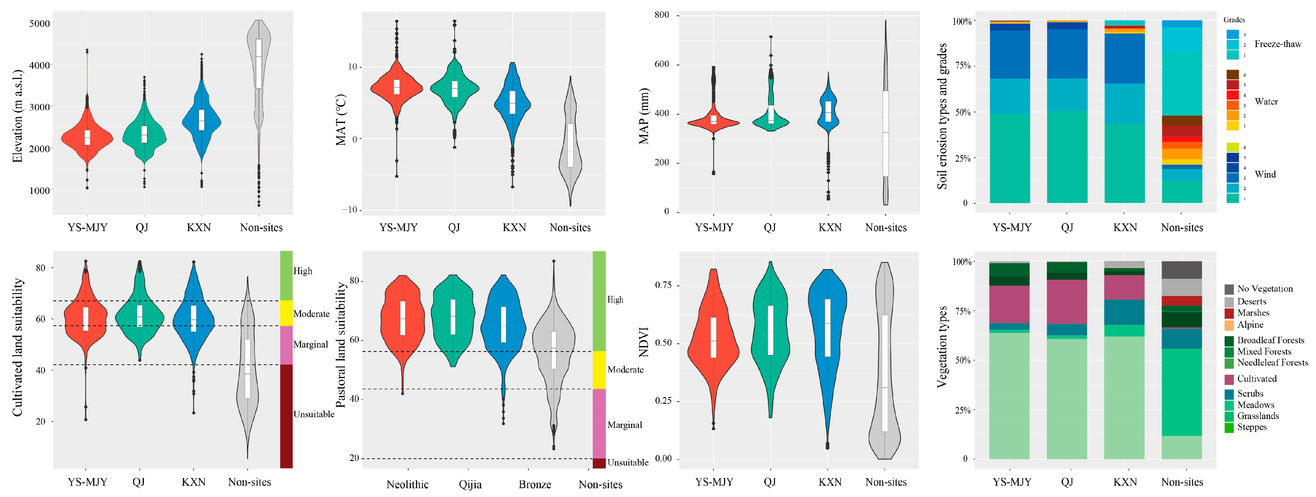
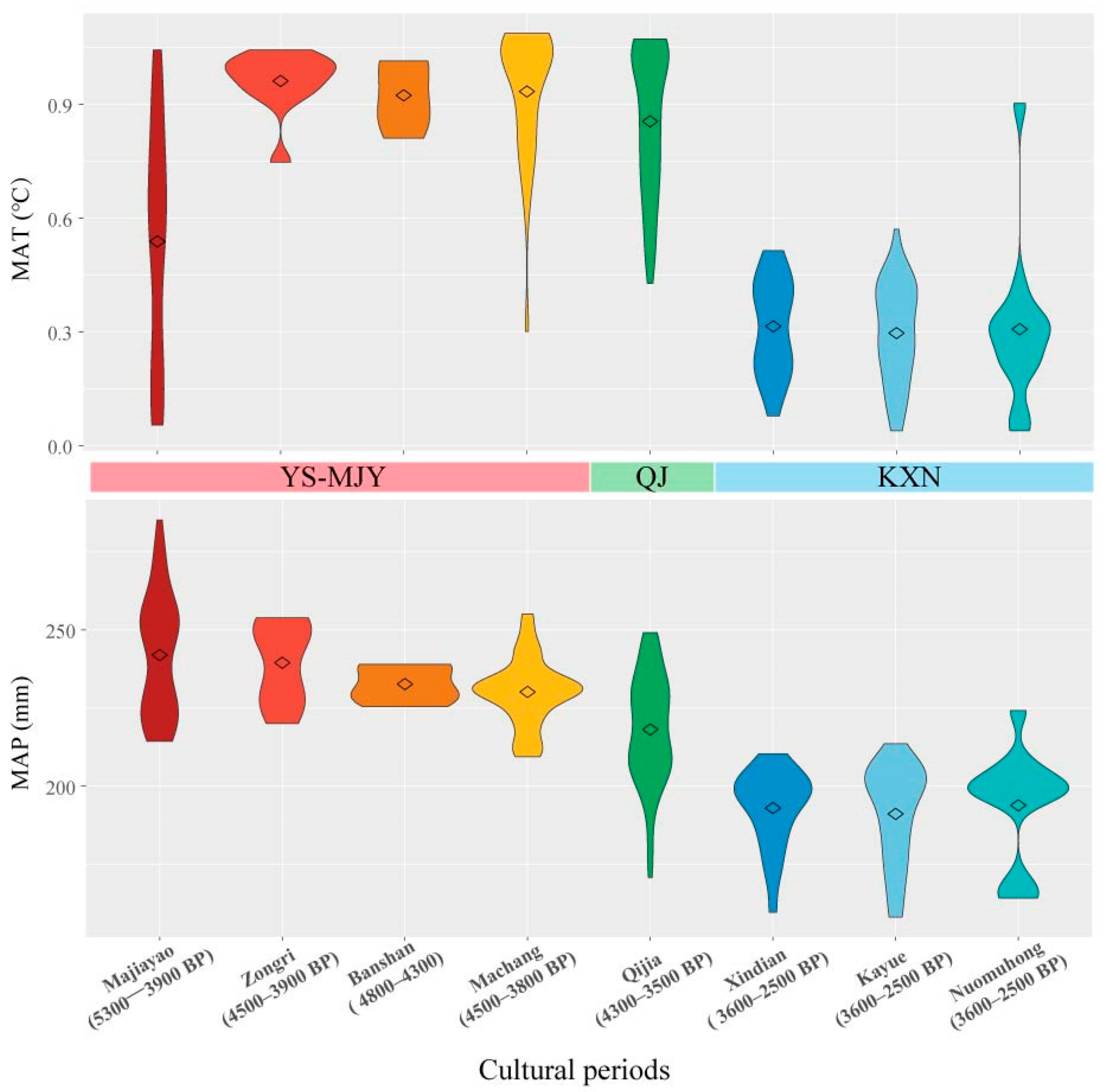
3.3. Geographic Factor Variation between Different Categories

The violin and box plots visually depict the distribution of six crucial variables for the various cultural phases and non-sites (Figure 6). Non-sites exhibited significant disparities, which represented environments that were excessively harsh for human survival. The elevation gradually increased across the different cultural stages, while the MAT decreased, and the MAP fluctuated around 400 mm. Soil erosion types displayed a distinguish boundary for sites and non-sites. The main sites were located in moderately cultivated land suitability areas. The NDVI showed a slight increase from the Neolithic to Bronze Age. Vegetation coverage revealed a decline in forest percentage from the Neolithic to the Bronze Age. At the same time, the pastoral area (steppe, grassland, meadow, shrub) increased, and the percentage of cultivated area decreased, according to current patterns (Figure 4).
The classification tree figure (Figure 7) exhibits the relationship between environment and culture. Soil erosion was a primary factor, serving as a “root” to effectively distinguish between most sites and non-sites. Elevation also played an important role, with a boundary of 3363 m to distinguish non-sites, and a boundary of 2489 m to distinguish KXN cultural sites. Below the 2489 m elevation limit, cultivated land suitability became crucial, with a threshold of 58 distinguishing between the YS-MJY and KXN cultures. These results provide strong archaeological interpretability and offer a more objective partition threshold than previous studies have.
The SOM method is an unsupervised method focusing on the geographic environments of sites, and sites with similar factors are grouped together. We analyzed all geographic variables and the four important variables, respectively, and generated almost identical results. The findings showed distinguished environmental boundaries in Figure 8. The YS-MJY, QJ, and KXN cultural sites almost coexisted with a lower elevation and suitable environments. Many KXN cultural sites were the first to break the boundary and to develop in high-elevation areas with harsher environments. Non-site points undoubtedly occupied cells in extremely harsh environments, further establishing a boundary between sites and non-sites.

4. Discussion

4.1. Environmental Selection Strategies across Different Cultural Stages

Archaeological culture is an assemblage of past artifacts and remnants sharing similar social features, and it encompasses artifacts and technology, subsistence economy, settlements, and burial patterns within a specific period and region [102]. The settlement locations of each type of culture always follow certain rules [103]. In the NETP, models show a strong connection between geographic environments and settlement locations. Based on traditional binary sites/non-sites APM, this study further explored the application of a multi-classification model in examining the environmental differences between cultural stages. The importance ranking of variables generated by the RF model offered a new insight for interpreting human environmental selection strategies.
The binary model for sites and non-sites revealed a clear human sensibility, as compared to random points located away from human settlements. The top five variables in the importance ranking were as follows: soil erosion > elevation > cultivated land suitability > precipitation > NDVI > vegetation type. Regarding the three-classification model for different stages, YS-MJY and QJ cultural sites exhibited lower accuracy. By combining the SOM results, we observed that YS-MJY, QJ, and part of the KXN cultural sites shared similar environmental strategies at lower elevations with a suitable environment and rich vegetational area, while the rest of the KXN cultural sites adapted to more challenging altitude environments. The top five variables in ranking were elevation > precipitation > cultivated land suitability > pastoral suitability > NDVI. This ranking suggests that the KXN culture primarily overcame these environmental limitations and exhibited new adaptations to some extent. All models indicated that elevation had great importance. This aligns with the fact that elevation largely dictates the local environment and sets the boundaries for human habitation in the NETP [71,104]. Cultivated land suitability also played an important role. This metric can even indicate the suitability for human habitation in an agricultural society [72]. Soil erosion was assigned greater weight in distinguishing between sites and non-sites because some special areas with water and freeze-thawing erosion are permanently uninhabitable. Although temperature was excluded from our models, it remains important for human settlements. Temperature is strongly correlated with elevation (R2 = 0.95). Numerous studies have demonstrated its crucial role in crop growth in the NETP, especially in the limited cultivation of millet in lower elevation valley zones [25,37,105,106,107]. Precipitation can also influence farming, vegetation, and land suitability. Human societies sensibly respond to climate change by selecting habitats adapted to their socioeconomic needs [108].
It should be noted that the present model was developed based on modern environmental datasets. This is critical because certain factors, such as vegetation, land suitability, and climate, have experienced instability over thousands of years. This challenge is commonly faced in all ancient simulations, as accurately reconstructing past surface environmental data is exceedingly difficult. Although some studies argue that slight changes in temporal environments can be ignored, our study considered this issue from the perspective of relative spatial differences. We highlighted the relative spatial differences in geographic environments, particularly in the NETP region where elevation dominated the environment. These differences were more robust in a stable climate system over the past millennia. According to quantitative climate reconstruction curves, temporal fluctuations matter less than spatial variance in the NETP [109,110]. ML methods also have the potential to identify these relative differences.
Additionally, data error may limit a precise analysis on micro topographies. In this study, slope, aspect, and curvature consistently ranked lower. This does not necessarily indicate their weak impact on settlement location, but the results may be limited by data precision. As a result, our study focuses on predicting site probabilities at a landscape scale rather than precisely identifying archaeological potential sites. The RF model can accept more geographic factors and provide an objective importance ranking. It encompasses high robustness as well as sensitivity to variable differences in classification [44,92]. For example, the slight differences in precipitation and cultivated land suitability between categories cannot be captured by a single factor comparison, but they may be captured by a higher ranking in RF models. However, tree-based algorithms focus on the effects of individual factors and may miss interactions between parameters. Although this may be conducive to the archeological interpretation of human behaviors, it may be less conducive to the accurate forecasting of archaeological potential. More AI or ML methods, such as popular deep learning methods and novel environmental data, could be explored to enhance model performance and to simulate complex or uncertain human–land relationships in the future [111,112].
Last but not least, it is undeniable that the database of the ‘Chinese Cultural Relic Atlas’ used in this study was obtained through archaeological surveys rather than systematic excavations. The quality and comprehensiveness of the data are finite. Some criticism has been raised regarding its rough cultural division and loose judgments on relics [113]. But the current understanding of cultural distribution from the Neolithic to the Bronze Age in the NETP is still within the framework of the ‘Chinese Cultural Relic Atlas’ data. Our analysis is indeed limited to the current archaeological knowledge available. The simulation results presented in this paper outlined a multistage process that aligns with current archaeological knowledge.

4.2. Socioeconomic and Climatic Changes Explain Settlements Dynamics in the NETP

The model results offer an objective but somewhat bland perspective, and it is crucial to interpret them in conjunction with practical archaeology. Previous studies have proposed several perspectives primarily focused on socioeconomic and climatic changes [24,28,35,36,114,115]. In the present study, we further analyzed this process by quantitively analyzing subsistence and climate dynamics across three cultural periods.
We utilized published data on 14C chronology, archaeological animal and plant remains, and reliable climate reconstruction data [109,110,116,117]. Each accurate 14C data range (95% confidence interval) was intersected with the climate curves derived from the Delingha tree ring MAP reconstruction and the TP simulated records of MAT [109,110]. The mean value of each fragment represents the climate context within one 14C age range. All climate fragments corresponding to 14C data ranges were attributed to each culture, and the results are displayed in Figure 9. This method presents the climate background of different cultures more accurately and intuitively and avoids the illusion of period comparison. The climate context exhibited distinct boundaries, with noticeable changes during the QJ cultural period that were characterized by a trend towards colder and drier conditions. This climate change pattern was verified at the regional and global scales as well [48,118,119,120,121]. Additionally, social subsistence economies were quantitatively analyzed using animal and plant remains through PCA and SOM, respectively (Figure 10). Obviously, subsistence strategies in the YS-MJY period were dominated by millet and wildlife resources. The QJ expanded this subsistence to include cattle and sheep livestock, and minor sites adopted barley and wheat agriculture. Most of the KXN sites shifted to barley- and wheat-dominated agriculture and pastoral subsistence. By combining the rules governing settlement location choices with temporal climate and social changes, we deduced the following dynamics in the human–environment interactions.
Neolithic YS-MJY cultural migrations introduced innovative technologies, including millet agriculture, painted pottery, and domesticated pigs around 5200 BP. They often interacted with indigenous foragers, who lived at higher elevations through trade and intermarriage [24,28,29]. On a regional scale, settlement locations were closely tied to agricultural practices and farmers engaged in year-round millet agricultural activities in the low elevation (<2500 m a.s.l.) area of Hehuang valley with suitable hydrothermal conditions [37]. Moreover, the YS-MJY cultural period had a warmer and wetter climatic context. This context was more conducive to agricultural development and also provided abundant wild resources. Zooarchaeological evidence revealed a high consumption of wild animals, along with scattered domestic pig remains [122,123]. The Shannashuzha sites in the marginal NETP even found tropical animal remains, revealing that the prevalence of high-intensity hunting persisted during the Majiaoyao period [123,124]. Therefore, YS-MJY cultural settlers selected landscapes with lower elevation and higher forest cover, which likely suggests a subsistence strategy based on millet cultivation and hunting of wild animals. Pollen and archaeological charcoal data also support the idea that YS-MJY period sites (before 4300 BP) had a high probability of being surrounded by forests [125,126,127].
The QJ culture inherited millet agriculture and developed an increasingly complex social structure. Its duration overlapped with the YS-MJY cultur due to inter-regional synchronized developments. New technologies, such as bronzeware, jade carving and architecture, and intricate social practices, such as graded burials, weapons, and sacrificial activities, developed during this period, reflecting the heightened social resilience of the QJ culture [53,57,128,129]. However, this period also faced climatic challenges due to the global 4.2 ka cold and dry climate events [62,63]. This period intensified competition for food resources and led to a decrease in millet planting probabilities based on ecological niche considerations [25]. Pollen evidence from Qinghai Lake and Caodalian Lake also indicates a transition from forest to grassland [125,126]. However, the number and distribution of sites were similar to those of the YS-MJY culture, suggesting that the QJ cultural living space was not in decline in the NETP. This is because trans-continental cultural exchange brought exotic barley and wheat crops, as well as cattle and sheep livestock, around 4000 BP [130]. The nearby locations and climatic deteriorations prompted the QJ cultural group to adopt novel subsistence strategies to alleviate population pressure. The adoption of barley and wheat was gradual, according to small site findings and later dates [131]. In contrast, the utilization of livestock, such as cattle and sheep, was rapid and widespread during this stage [132]. Climate change potentially led to a decline in wild animals, which would have made the novel domesticated animals more appealing. Hence, the pastoral subsistence economy emerged early, likely as a supplement to millet-based economies, thus supporting the QJ cultural people in resisting climate change. Ethnography suggests that today’s high-altitude groups utilize similar strategies, engaging in animal husbandry to supplement agriculture [133].
After 3600 BP, the uniform culture broke up into several branches of Kayue, Xindian, and Nuomuhong (KXN) cultures. Although the climate continued to be cold and dry, the adaptations to cold-tolerant barley wheat and cattle sheep supported humans in breaking the previous elevation constraint of ~2500 m, thus enabling them to settle in more extreme environments [24,121]. Horse and yak utilization further promoted social resilience [61,134,135,136]. This occupation occurred around 3600 BP, but it was not sudden, and it involved a prolonged period of preparation. Bronze Age people occupied more grasslands and high pastoral land suitability patches, probably for pasturing purposes. It is worth noting that climate still limited millet agriculture to low-elevation valleys. For example, many Xindian cultural sites persisted with millet agriculture in valley areas due to dietary traditions [137]. A special group known as the Nuomuhong culture abandoned agriculture and instead developed a nomadic pastoral economy in the margins of the arid Qaidam Basin [61].
In summary, these settlement dynamics reflect intricate social responses to geographic environments, validating the latest “gear” theory [37]. This study presents a detailed process of human–environment interactions that demonstrate a synergy involving the effect of multiple factors, primarily geography and social subsistence, in the locations of settlement sites.

5. Conclusions

This study presents a novel methodological exploration and emphasizes the advantages of machine learning in addressing the complex relationship between the environment and settlements. The binary RF model (distinguishing between sites and non-sites) revealed a strong correlation between settlement location and the surrounding environment, thus enabling predictions of archaeological probabilities at a landscape scale across the NETP. The three-classification RF model (three cultural periods) showed distinguishable environmental selection strategies from the Neolithic to the Bronze Age. The model-generated importance rankings and the classification tree highlighted the crucial roles that elevation, cultivated land suitability, precipitation, and soil erosion types play in shaping human environmental strategies across different cultural periods.
To further interpret the underlying mechanisms of human environmental strategies, a quantitative analysis encompassing temporal change in climate and social subsistence was undertaken. The results highlight the synergistic influence that factors related to social organization and geography had on settlement selection. The YS-MJY cultural (5500–4000 BP) settlements were located in low-altitude areas with suitable hydrothermal conditions; these factors aligned with the millet agriculture system and the preference for wild resources. The QJ culture (4300–3600 BP) was early to accept cattle and sheep livestock as a supplement, which helped them resist global climatic deterioration. This transitional period also prepared the people for the larger-scale occupation of high-altitude areas after 3600 BP.

Supplementary Materials

The following supporting information can be downloaded at: https://0-www-mdpi-com.brum.beds.ac.uk/article/10.3390/rs16081454/s1, Figure S1: Modern land coverage types in the Tibetan Plateau [138]; Figure S2: Suitability ordered class and distribution of cultivated and pastoral land in the modern Tibetan Plateau; Figure S3: Dependent variables Pearson correlation heat map; Figure S4: The importance rankings and OOB confusion matrix for the three-classification model (YS-MJY, QJ, and KXN cultures) and the binary classification model (sites and non-sites); Table S1: The whole results of 10-fold CV, repeat 5 times.

Author Contributions

Conceptualization, G.L., J.D. and G.D.; methodology, G.L. and M.C.; validation, J.D., J.F. and X.W.; formal analysis, J.D. and X.W.; investigation, J.D., M.C. and X.W.; resources, J.D.; data curation, J.D.; writing—original draft preparation, G.L. and G.D.; writing—review and editing, J.D. and X.W.; visualization, G.L. and J.D.; funding acquisition, G.D. All authors have read and agreed to the published version of the manuscript.

Funding

This research was funded by NSFC-INSF Joint Research Project (Grant No. 42261144670); the Second Tibetan Plateau Scientific Expedition and Research Program (2019QZKK0601); the Academician and Expert Workstation of Yunnan Province (202305AF150183) and the European Research Council Grant (ERC-2019-ADG-883700-TRAM).

Data Availability Statement

All R scripts used to generate and evaluate the models in this study have been deposited in GitHub (https://github.com/ligangdongjiajia/archaeological-potential-predicting-Using-RF-in-NETP-main-code.git, accessed on 10 April 2024).

Acknowledgments

We would like to express our gratitude to Shanjia Zhang at Lanzhou University for his valuable assistance in structuring the article. We also extend our thanks to Yishi Yang at Gansu Provincial Institute of Cultural Relics and Archaeology for helping us comb the cultural lineage of the NETP. Additionally, we extend our thanks to Daniel Petticord at the University of Cornell for his support in English language editing and grammatical refinement of the manuscript.

Conflicts of Interest

The authors declare no conflicts of interest.

References

  1. Fernandes, R.; Geeven, G.; Soetens, S.; Klontza-Jaklova, V. Deletion/Substitution/Addition (DSA) model selection algorithm applied to the study of archaeological settlement patterning. J. Archaeol. Sci. 2011, 38, 2293–2300. [Google Scholar] [CrossRef]
  2. Graves, D. The use of predictive modelling to target neolithic settlement and occupation activity in Mainland Scotland. J. Archaeol. Sci. 2011, 38, 633–656. [Google Scholar] [CrossRef]
  3. Wachtel, I.; Zidon, R.; Garti, S.; Shelach-Lavi, G. Predictive modeling for archaeological site locations: Comparing Logistic Regression and Maximal Entropy in north Israel and north-east China. J. Archaeol. Sci. 2018, 92, 28–36. [Google Scholar] [CrossRef]
  4. Koohpayma, J.; Makki, M.; Lentschke, J.; AlaviPanah, S.K. Predicting potential locations of ancient settlements using GIS and Weights-Of-Evidence Method (case study: North-east of Iran). J. Archaeol. Sci. Rep. 2021, 40, 103229. [Google Scholar] [CrossRef]
  5. Yan, L.; Lu, P.; Chen, P.; Danese, M.; Li, X.; Masini, N.; Wang, X.; Guo, L.; Zhao, D. Towards an operative predictive model for the Songshan Area during the Yangshao period. Int. J. Geo-Inf. 2021, 10, 217. [Google Scholar] [CrossRef]
  6. Tan, B.; Wang, H.; Wang, X.; Yi, S.; Zhou, J.; Ma, C.; Dai, X. The study of early human settlement preference and settlement prediction in Xinjiang, China. Sci. Rep. 2022, 12, 5072. [Google Scholar] [CrossRef] [PubMed]
  7. Tan, L.; Wu, B.; Zhang, Y.; Zhao, S. GIS-Based precise predictive model of Mountain Beacon Sites in Wenzhou, China. Sci. Rep. 2022, 12, 10773. [Google Scholar] [CrossRef] [PubMed]
  8. Danese, M.; Masini, N.; Biscione, M.; Lasaponara, R. Predictive modeling for preventive archaeology: Overview and case study. Open Geosci. 2014, 6, 42–55. [Google Scholar] [CrossRef]
  9. Caracausi, S.; Berruti, G.L.F.; Daffara, S.; Bertè, D.; Rubat Borel, F. Use of a GIS predictive model for the identification of high altitude prehistoric human frequentations. Results of the Sessera Valley project (piedmont, Italy). Quat. Int. 2018, 490, 10–20. [Google Scholar] [CrossRef]
  10. Wu, H.; Wang, X.; Wang, X.; Zhang, L.; Dong, S. Predictive modeling for Neolithic settlements in the Lingnan Region, South China. J. Archaeol. Sci. Rep. 2023, 49, 103992. [Google Scholar] [CrossRef]
  11. Guo, F. Study of Archaeological Sites Predictive Distribution Based on Logistic Regression Optimization Method—A Cast Study of Fenhe River Basin. Master’s Thesis, Institute of Remote Sensing and Digital Earth Chinese Academy of Sciences, Beijing, China, 2018. [Google Scholar]
  12. Liu, Y. Simulation of Prehistoric Agriculture Dispersal Routes on the Tibetan Plateau Based on Explainable Machine Learning. Master’s Thesis, Lanzhou University, Lanzhou, China, 2023. [Google Scholar]
  13. Kvamme, K.L. Computer processing techniques for regional modeling of archaeological site locations. Adv. Comput. Archaeol. 1983, 1, 26–52. [Google Scholar]
  14. Kvamme, K.L. A predictive site location model on the High Plains: An example with an independent test. Plains Anthropol. 1992, 37, 19–40. [Google Scholar] [CrossRef]
  15. Ni, J. Predictive model of archaeological sites in the upper reaches of the Shuhe River in Shandong. Prog. Geogr. Sci. 2009, 28, 489–493. [Google Scholar]
  16. Han, Y. Research on the Relationship between Human and Environment in Jinghe River Basin during Pre-Qin Period Supported by Geographic Information Technology. Master’s Thesis, Northwest University, Xian, China, 2020. [Google Scholar]
  17. Cao, J.; Zhang, Z.; Du, J.; Zhang, L.; Song, Y.; Sun, G. Multi-geohazards susceptibility mapping based on machine learning—A case study in Jiuzhaigou, China. Nat. Hazards 2020, 102, 851–871. [Google Scholar] [CrossRef]
  18. Zheng, X.; He, G.; Wang, S.; Wang, Y.; Wang, G.; Yang, Z.; Yu, J.; Wang, N. Comparison of machine learning methods for potential active landslide hazards identification with multi-source data. Int. J. Geo-Inf. 2021, 10, 253. [Google Scholar] [CrossRef]
  19. Cao, W.; Pan, D.; Xu, Z.; Zhang, W.; Ren, Y.; Nan, T. Landslide disaster vulnerability mapping study in Henan Province: Comparison of different machine learning models. Bull. Geol. Sci. Technol. 2023. [Google Scholar] [CrossRef]
  20. Mao, K.; Zhang, C.; Shi, J.; Wang, X.; Guo, Z.; Li, C.; Dong, L.; Wu, M.; Sun, R.; Wu, S.; et al. The paradigm theory and judgment conditions of geophysical parameter retrieval based on artificial intelligence. Smart Agric. 2023, 5, 161–171. [Google Scholar] [CrossRef]
  21. Mao, K.; Yuan, Z.; Shi, J.; Wu, S.; Hu, D.; Che, J.; Dong, L. Theory and engineering technology implementation of Artificial Intelligence retrieval paradigm for parameters of remote sensing based on Big Data. J. Agric. Big Data 2023, 5, 1–12. [Google Scholar] [CrossRef]
  22. Zheng, Q.; Tian, X.; Yu, Z.; Jiang, N.; Elhanashi, A.; Saponara, S. Application of wavelet-packet transform driven deep learning method in PM2. 5 concentration prediction: A case study of Qingdao, China. Sustain. Cities Soc. 2023, 92, 104486. [Google Scholar] [CrossRef]
  23. Zheng, Q.; Tian, X.; Yu, Z.; Jin, B.; Jiang, N.; Ding, Y.; Yang, M.; Elhanashi, A.; Saponara, S.; Kpalma, K. Application of complete ensemble empirical mode decomposition based multi-stream informer (CEEMD-MsI) in PM2.5 concentration long-term prediction. Expert. Syst. Appl. 2024, 245, 123008. [Google Scholar] [CrossRef]
  24. Chen, F.; Dong, G.; Zhang, D.; Liu, X.; Jia, X.; An, C.; Ma, M.; Xie, Y.; Barton, L.; Ren, X.; et al. Agriculture facilitated permanent human occupation of the Tibetan Plateau after 3600 B.P. Science 2015, 347, 248–250. [Google Scholar] [CrossRef] [PubMed]
  25. d’Alpoim Guedes, J.; Manning, S.W.; Bocinsky, R.K. A 5500-Year model of changing crop niches on the Tibetan Plateau. Cur. Anthropol. 2016, 57, 517–522. [Google Scholar] [CrossRef]
  26. Wang, H.; Yang, M.A.; Wangdue, S.; Lu, H.; Chen, H.; Li, L.; Dong, G.; Tsring, T.; Yuan, H.; He, W.; et al. Human genetic history on the Tibetan Plateau in the past 5100 years. Sci. Adv. 2023, 9, eadd5582. [Google Scholar] [CrossRef]
  27. Zhao, Y.; Obie, M.; Stewart, B.A. The archaeology of human permanency on the Tibetan Plateau: A critical review and assessment of current models. Quat. Sci. Rev. 2023, 313, 108211. [Google Scholar] [CrossRef]
  28. Ma, M.; Dong, G.; Jia, X.; Wang, H.; Cui, Y.; Chen, F. Dietary shift after 3600 cal yr BP and its influencing factors in northwestern China: Evidence from stable isotopes. Quat. Sci. Rev. 2016, 145, 57–70. [Google Scholar] [CrossRef]
  29. Ren, L.; Dong, G.; Liu, F.; d’Alpoim-Guedes, J.; Flad, R.K.; Ma, M.; Li, H.; Yang, Y.; Liu, Y.; Zhang, D.; et al. Foraging and farming: Archaeobotanical and zooarchaeological evidence for neolithic exchange on the Tibetan Plateau. Antiquity 2020, 94, 637–652. [Google Scholar] [CrossRef]
  30. Lu, H. Local millet farming and permanent occupation on the Tibetan Plateau. Sci. China Earth Sci. 2023, 66, 430–434. [Google Scholar] [CrossRef]
  31. Danese, M.; Masini, N.; Biscione, M.; Lasaponara, R. GIS and archaeology: A spatial predictive model for Neolithic sites of the Tavoliere (Apulia). In Proceedings of the First International Conference on Remote Sensing and Geoinformation of Environment, Paphos, Cyprus, 8–10 August 2013; Volume 8795, pp. 146–155. [Google Scholar]
  32. Vaughn, S.; Crawford, T. A predictive model of archaeological potential: An example from northwestern Belize. Appl. Geogr. 2009, 29, 542–555. [Google Scholar] [CrossRef]
  33. Wang, L.; Yang, Y.; Jia, X. Hydrogeomorphic settings of late Paleolithic and early-mid Neolithic sites in relation to subsistence variation in Gansu and Qinghai Provinces, northwest China. Quat. Int. 2016, 426, 18–25. [Google Scholar] [CrossRef]
  34. Ma, M.; Dong, G.; Jia, X.; Zhang, Z. Analysis of settlement patterns during Neolithic and Bronze period and its influencing factors in Hualong county, Qinghai Province, China. Quat. Sci. 2012, 32, 209–218. [Google Scholar] [CrossRef]
  35. Hou, G.; Xu, C.; Xiao, J. Comparative analysis of Prehistoric sites distribution around 4 ka B.P. in Gansu-Qinghai region based on GIS. Sci. Geogr. Sin. 2012, 32, 116–120. [Google Scholar] [CrossRef]
  36. Dong, G.; Du, L.; Liu, R.; Li, Y.; Chen, F. Human-environment interaction systems between regional and continental scales in mid-latitude Eurasia during 6000–3000 years ago. Innov. Geosci. 2023, 1, 100038. [Google Scholar] [CrossRef]
  37. d’Alpoim Guedes, J. Did foragers adopt farming? A perspective from the margins of the Tibetan Plateau. Quat. Int. 2018, 489, 91–100. [Google Scholar] [CrossRef]
  38. Ma, Z.; Song, J.; Wu, X.; Hou, G.; Huan, X. Spatiotemporal distribution and geographical impact factors of barley and wheat during the late Neolithic and Bronze Age (4000–2300 cal. a BP) in the Gansu–Qinghai region, northwest China. Sustainability 2022, 14, 5417. [Google Scholar] [CrossRef]
  39. Chen, X.; Lü, H.; Liu, X.; Frachetti, M.D. Geospatial modelling of farmer–herder interactions maps cultural geography of Bronze and Iron Age Tibet, 3600–2200 BP. Sci. Rep. 2024, 14, 2010. [Google Scholar] [CrossRef] [PubMed]
  40. Zhu, Y.; Hou, G.; Lancuo, Z.; Gao, J.; Pang, L. GIS-based analysis of traffic routes and regional division of the Qinghai-Tibetan Plateau in prehistoric period. Prog. Geogr. 2018, 37, 438–449. [Google Scholar] [CrossRef]
  41. Hou, G.; Lancuo, Z.; Zhu, Y.; Pang, L. Communication route and its evolution on the Qinghai-Tibet Plateau during the prehistoric time. Acte Geogr. Sin. 2021, 76, 1294–1313. [Google Scholar] [CrossRef]
  42. Lancuo, Z.; Hou, G.; Xu, C.; Jiang, Y.; Wang, W.; Gao, J.; Wende, Z. Simulation of exchange routes on the Qinghai-Tibetan Plateau shows succession from the neolithic to the Bronze Age and strong control of the physical environment and production mode. Front. Earth Sci. 2023, 10, 1079055. [Google Scholar] [CrossRef]
  43. Velasquez, M.; Hester, P.T. An analysis of multi-criteria decision making methods. Int. J. Oper. Res. 2013, 10, 56–66. [Google Scholar]
  44. Rhys, H.I. Machine Learning with R, the Tidyverse, and mlr; Manning Publications: New York, NY, USA, 2020. [Google Scholar]
  45. Li, Y.; Zhu, G. Changes of climate zones in the transition area of three natural zones during the past 50 years an their responses to climate change. Adv. Earth Sci. 2015, 30, 791–801. [Google Scholar] [CrossRef]
  46. Zheng, D.; Zhao, D. Characteristics of natural environment of the Tibetan Plateau. Sci. Technol. Rev. 2017, 35, 13–22. [Google Scholar] [CrossRef]
  47. Zhang, Y.; Li, B.; Zheng, D. A discussion on the boundary and area of the Tibetan Plateau in China. Geogr. Res. 2002, 21, 1–8. [Google Scholar]
  48. Chen, F.; Zhang, J.; Liu, J.; Cao, X.; Hou, J.; Zhu, L.; Xu, X.; Liu, X.; Wang, M.; Wu, D. Climate change, vegetation history, and landscape responses on the Tibetan Plateau during the Holocene: A comprehensive review. Quat. Sci. Rev. 2020, 243, 106444. [Google Scholar] [CrossRef]
  49. Liu, X.; Jones, P.J.; Motuzaite Matuzeviciute, G.; Hunt, H.V.; Lister, D.L.; An, T.; Przelomska, N.; Kneale, C.J.; Zhao, Z.; Jones, M.K. From ecological opportunism to multi-cropping: Mapping food globalisation in Prehistory. Quat. Sci. Rev. 2019, 206, 21–28. [Google Scholar] [CrossRef]
  50. Dong, G.; Du, L.; Yang, L.; Lu, M.; Qiu, M.; Li, H.; Ma, M.; Chen, F. Dispersal of crop-livestock and geographical-temporal variation of subsistence along the steppe and Silk Roads across Eurasia in Prehistory. Sci. China Earth Sci. 2022, 65, 1187–1210. [Google Scholar] [CrossRef]
  51. Wang, H. The pedigree and pattern of Neolithic-Bronze Age archaeological culture in Gansu-Qinghai area. Collect. Stud. Archaeol. 2012, 21, 210–243. [Google Scholar]
  52. Chen, H.; Wang, G.; Mei, D.; Suo, N. Excavation briefing of Zongri Site in Tongde County, Qinghai Province. Archaeology 1998, 44, 1–14. [Google Scholar]
  53. Womack, A.; Flad, R.; Zhou, J.; Brunson, K.; Toro, F.H.; Su, X.; Hein, A.; d’Alpoim Guedes, J.; Jin, G.; Wu, X.; et al. The Majiayao to Qijia transition: Exploring the intersection of technological and social continuity and change. Asian Archaeol. 2021, 4, 95–120. [Google Scholar] [CrossRef]
  54. Wei, W.; Tang, S. Qijia Culture Hundred Years Research Article; Lanzhou University Press: Lanzhou, China, 2020. [Google Scholar]
  55. Li, Y.; Lu, P.; Mao, L.; Chen, P.; Yan, L.; Guo, L. Mapping spatiotemporal variations of Neolithic and Bronze Age settlements in the Gansu-Qinghai region, China: Scale grade, chronological development, and social organization. J. Archaeol. Sci. 2021, 129, 105357. [Google Scholar] [CrossRef]
  56. Chen, G. The community practicing metallurgy amidst the Xichengyi and Qijia: Preliminary study on early metallurgical population and related problems in Hexi Corridor. Archaeol. Cult. Relics 2017, 5, 37–44. [Google Scholar]
  57. Ren, R.; Chen, W. Some basic questions about Qijia culture. Sichuan Cult. Relics 2017, 195, 72–82. [Google Scholar]
  58. Wang, L. Scientific Study on Early Copper and Bronze Objects in the Gansu-Qinghai Region: With a Focus on the Mogou Site in Lintan. Ph.D. Thesis, University of Science and Technology Beijing, Beijing, China, 2018. [Google Scholar]
  59. Zhen, Q. A study on large-double-ear pottery jars from Qijia culture and related sites. Sichuan Cult. Relics 2020, 213, 34–51. [Google Scholar]
  60. Jia, X. Cultural Evolution Process and Plant Remains during Neolithic-Bronze Age in Northeast Qinghai Province. Ph.D. Thesis, Lanzhou University, Lanzhou, China, 2012. [Google Scholar]
  61. Dong, G.; Ren, L.; Jia, X.; Liu, X.; Dong, S.; Li, H.; Wang, Z.; Xiao, Y.; Chen, F. Chronology and subsistence strategy of Nuomuhong culture in the Tibetan Plateau. Quat. Int. 2016, 426, 42–49. [Google Scholar] [CrossRef]
  62. An, C.; Feng, Z.; Tang, L. Evidence of a humid Mid-Holocene in the western part of Chinese Loess Plateau. Sci. Bull. 2003, 48, 2472–2479. [Google Scholar] [CrossRef]
  63. An, C.; Feng, Z.; Tang, L.; Chen, F. Environmental changes and cultural transition at 4 cal. ka BP in central Gansu. Acte Geogr. Sin. 2003, 58, 743–748. [Google Scholar]
  64. Bureau of National Cultural Relics. Atlas of Chinese Cultural Relics—Fascicule of Qinghai Province; Sinomap Press: Beijing, China, 1996. [Google Scholar]
  65. Bureau of National Cultural Relics. Atlas of Chinese Cultural Relics—Fascicule of Gansu Province; Sinomap Press: Beijing, China, 2011. [Google Scholar]
  66. Hosner, D.; Wagner, M.; Tarasov, P.E.; Chen, X.; Leipe, C. Spatiotemporal distribution patterns of archaeological sites in China during the Neolithic and Bronze Age: An overview. Holocene 2016, 26, 1576–1593. [Google Scholar] [CrossRef]
  67. Gu, X. A Study on the Relationship between Majiayao Cultural Residence and Tomb Space. Master’s Thesis, Lanzhou University, Lanzhou, China, 2020. [Google Scholar]
  68. Li, Y. Discussion on the burial customs of prehistoric settlements in China. Cult. Relics Cent. China 2017, 06, 39–44+51. [Google Scholar]
  69. Liu, X. Burial practices of the Cayo culture. J. Qinghai Norm. Univ. Soc. Sci. 1995, 65, 115–119. [Google Scholar] [CrossRef]
  70. Cooke, R.U.; Johnson, J.H. Trends in Geography: An Introductory Survey; Pergamon Press: Oxford, UK, 1969. [Google Scholar]
  71. Meyer, M.C.; Aldenderfer, M.S.; Wang, Z.; Hoffmann, D.L.; Dahl, J.A.; Degering, D.; Haas, W.R.; Schlütz, F. Permanent human occupation of the central Tibetan Plateau in the early Holocene. Science 2017, 355, 64–67. [Google Scholar] [CrossRef]
  72. Yao, M.; Shao, D.; Lv, C.; An, R.; Gu, W.; Zhou, C. Evaluation of arable land suitability based on the suitability function—A case study of the Qinghai-Tibet Plateau. Sci. Total Environ. 2021, 787, 147414. [Google Scholar] [CrossRef]
  73. Jenks, G.F. The data model concept in statistical mapping. Int. Yearb. Cartogr. 1967, 7, 186–190. [Google Scholar]
  74. Xu, X. [Dataset] Spatial Distribution Dataset of Annual Vegetation Index (NDVI) in China; Resource and Environmental Science Data Registration and Publication System: Beijing, China, 2018; Available online: https://www.resdc.cn/DOI/doi.aspx?DOIid=49 (accessed on 10 January 2024).
  75. Yao, M. [Dataset] Grading Map of Agricultural Suitability on the Tibet Plateau (2018); National Tibetan Plateau/Third Pole Environment Data Center: Beijing, China, 2019. [Google Scholar] [CrossRef]
  76. ADC World Map. [Dataset] Third Pole 1:1 Million System Data Set (2014); National Tibetan Plateau Data Center: Beijing, China, 2019. [Google Scholar]
  77. Zhang, G. [Dataset] Dataset of All Lakes on the Tibetan Plateau (2000); National Tibetan Plateau Data Center: Beijing, China, 2019. [Google Scholar] [CrossRef]
  78. Ding, M. [Dataset] Temperature and Precipitation Grid Data of the Qinghai Tibet Plateau and Its Surrounding Areas in 1998–2017 Grid Data of Annual Temperature and Annual Precipitation on the Tibetan Plateau and Its Surrounding Areas during 1998–2017; National Tibetan Plateau/Third Pole Environment Data Center: Beijing, China, 2019. [Google Scholar] [CrossRef]
  79. Qin, F.; Zhao, Y.; Cao, X. Biome reconstruction on the Tibetan Plateau since the Last Glacial Maximum using a machine learning method. Sci. China: Earth Sci. 2022, 65, 518–535. [Google Scholar] [CrossRef]
  80. RStudio Team. RStudio: Integrated Development Environment for R; Version 2023.09.1 +494; RStudio Team: Boston, MA, USA, 2020. [Google Scholar]
  81. R Development Core Team. R: A Language and Environment for Statistical Computing; R Foundation for Statistical Computing: Vienna, Austria, 2019. [Google Scholar]
  82. Kuhn, M. Building predictive models in R using the caret package. J. Stat. Softw. 2008, 28, 1–26. [Google Scholar] [CrossRef]
  83. Wickham, H.; Averick, M.; Bryan, J.; Chang, W.; McGowan, L.D.; François, R.; Grolemund, G.; Hayes, A.; Henry, L.; Hester, J.; et al. Welcome to the tidyverse. J. Open Source Softw. 2019, 4, 1686. [Google Scholar] [CrossRef]
  84. Bischl, B.; Lang, M.; Kotthoff, L.; Schiffner, J.; Richter, J.; Studerus, E.; Casalicchio, G.; Jones, Z.M. mlr: Machine learning in R. J. Mach. Learn. Res. 2016, 17, 1–5. Available online: https://jmlr.org/papers/v17/15-066.html (accessed on 14 April 2024).
  85. Probst, P.; Au, Q.; Casalicchio, G.; Stachl, C.; Bischl, B. Multilabel Classification with R Package mlr. arXiv 2017, arXiv:1703.08991. [Google Scholar] [CrossRef]
  86. Wehrens, R.; Kruisselbrink, J. Flexible self-organizing maps in kohonen 3.0. J. Stat. Softw. 2018, 87, 1–18. [Google Scholar] [CrossRef]
  87. Wehrens, R.; Buydens, L.M.C. Self-and super-organizing maps in R: The kohonen Package. J. Stat. Softw. 2007, 21, 1–19. [Google Scholar] [CrossRef]
  88. Bivand, R.S.; Pebesma, E.; Gómez-Rubio, V. Applied Spatial Data Analysis with R, 2nd ed.; Springer: New York, NY, USA, 2013. [Google Scholar]
  89. Hijmans, R.J. Raster: Geographic data analysis and modeling (raster 4.3.2). R. Package Version 2018, 2, 18. [Google Scholar]
  90. Loh, W.Y. Classification and regression trees. Wiley Interdiscipl. Rev. Data Min. Knowl. Discov. 2011, 1, 14–23. [Google Scholar] [CrossRef]
  91. Lantz, B. Machine Learning with R; Packt Publishing: Birmingham, UK, 2019. [Google Scholar]
  92. Breiman, L. Random forests. Mach. Learn. 2001, 45, 5–32. [Google Scholar] [CrossRef]
  93. Hutter, F.; Kotthoff, L.; Vanschoren, J. Automated Machine Learning: Methods, Systems, Challenges; Springer: Cham, Switzerland, 2019; pp. 3–33. [Google Scholar]
  94. Ben-David, A. About the relationship between ROC curves and Cohen’s kappa. Eng. Appl. Artif. Intell. 2008, 21, 874–882. [Google Scholar] [CrossRef]
  95. Fawcett, T. An introduction to ROC analysis. Pattern Recognit. Lett. 2006, 27, 861–874. [Google Scholar] [CrossRef]
  96. Hand, D.J.; Till, R.J. A simple generalisation of the area under the ROC curve for multiple class classification problems. Mach. Learn. 2001, 45, 171–186. [Google Scholar] [CrossRef]
  97. Kvamme, K.L. There and back again: Revisiting archaeological locational modeling. In GIS and Archaeological Site Location Modeling, 1st ed.; Mehrer, M.W., Wescot, K.L., Eds.; CRC Press: New York, NY, USA, 2006; pp. 3–38. [Google Scholar]
  98. Kohonen, T.; Oja, E.; Lehtio, P. Storage and processing of information in distributed associative memory systems. In Parallel Models of Associative Memory; Hinton, G.E., Anderson, J.A., Eds.; Psychology Press: New York, NY, USA, 1981; pp. 129–167. [Google Scholar]
  99. Vesanto, J.; Himberg, J.; Alhoniemi, E.; Parhankangas, J. Self-organizing map in Matlab: The SOM toolbox. In Proceedings of the Matlab DSP Conference, Tampere, Finland, 16–17 November 1999; Volume 99, pp. 16–17. [Google Scholar]
  100. Kohonen, T. Essentials of the self-organizing map. Neural Netw. 2013, 37, 52–65. [Google Scholar] [CrossRef] [PubMed]
  101. Lu, P.; Tian, Y.; Yang, R. The study of size-grade of Prehistoric settlements in the Circum-Songshan area based on SOFM network. J. Geogr. Sci. 2013, 23, 538–548. [Google Scholar] [CrossRef]
  102. Schein, E.H. Organizational Culture and Leadership, 2nd ed.; Jossey Bass Publishers: San Francisco, CA, USA, 1992. [Google Scholar]
  103. Smith, M.E.; Lobo, J.; Peeples, M.A.; York, A.M.; Stanley, B.W.; Crawford, K.A.; Gauthier, N.; Huster, A.C. The persistence of ancient settlements and urban sustainability. Proc. Natl. Acad. Sci. USA 2021, 118, e2018155118. [Google Scholar] [CrossRef]
  104. Cao, H.; Dong, G. Social development and living environment changes in the northeast Tibetan Plateau and contiguous regions during the late Prehistoric period. Reg. Sustain. 2020, 1, 59–67. [Google Scholar] [CrossRef]
  105. d’Alpoim Guedes, J.A.; Lu, H.; Hein, A.M.; Schmidt, A.H. Early Evidence for the use of wheat and barley as staple crops on the margins of the Tibetan Plateau. Proc. Natl. Acad. Sci. USA 2015, 112, 5625–5630. [Google Scholar] [CrossRef]
  106. Ma, W. Evaluation of Impact of Climate Change on Highland Barley Cultivation in Qinghai-Tibet Plateau. Ph.D. Thesis, Qinghai Normal University, Xining, China, 2022. [Google Scholar]
  107. d’Alpoim Guedes, J.A. Rethinking the spread of agriculture to the Tibetan Plateau. Holocene 2015, 25, 1498–1510. [Google Scholar] [CrossRef]
  108. Liu, J.; Xin, Z.; Huang, Y.; Yu, J. Climate suitability assessment on the Qinghai-Tibet Plateau. Sci. Total Environ. 2022, 816, 151653. [Google Scholar] [CrossRef] [PubMed]
  109. Yang, B.; Qin, C.; Bräuning, A.; Osborn, T.J.; Trouet, V.; Ljungqvist, F.C.; Esper, J.; Schneider, L.; Grießinger, J.; Büntgen, U.; et al. Long-term decrease in Asian monsoon rainfall and abrupt climate change events over the past 6700 years. Proc. Natl. Acad. Sci. USA 2021, 118, e2102007118. [Google Scholar] [CrossRef] [PubMed]
  110. Zhang, C.; Zhao, C.; Yu, S.-Y.; Yang, X.; Cheng, J.; Zhang, X.; Xue, B.; Shen, J.; Chen, F. Seasonal imprint of Holocene temperature reconstruction on the Tibetan Plateau. Earth-Sci. Rev. 2022, 226, 103927. [Google Scholar] [CrossRef]
  111. Huang, J.; Ma, H.; Sedano, F.; Lewis, P.; Liang, S.; Wu, Q.; Su, W.; Zhang, X.; Zhu, D. Evaluation of regional estimates of winter wheat yield by assimilating three remotely sensed reflectance datasets into the coupled WOFOST–PROSAIL model. Eur. J. Agron. 2019, 102, 1–13. [Google Scholar] [CrossRef]
  112. Mao, Y.; Sun, R.; Wang, J.; Cheng, Q.; Kiong, L.C.; Ochieng, W.Y. New time-differenced carrier phase approach to GNSS/INS integration. GPS Solut. 2022, 26, 122. [Google Scholar] [CrossRef]
  113. Zhu, N.; Wang, H.; Ma, Y. (Eds.) The Paper Collection of International Seminar on Qijia Culture and Huaxia Civilization. In Proceedings of the International Seminar on Qijia Culture and Huaxia Civilization, Guanghe, China, 1–2 August 2015; Culture Relics Press: Beijing, China, 2016. [Google Scholar]
  114. Brantingham, P.J.; Gao, X. Peopling of the northern Tibetan plateau. World Archaeol. 2006, 38, 387–414. [Google Scholar] [CrossRef]
  115. Ren, L.; Yang, Y.; Wang, Q.; Zhang, S.; Chen, T.; Cui, Y.; Wang, Z.; Liang, G.; Dong, G. The transformation of cropping patterns 642 from late Neolithic to early Iron Age (5900–2100 BP) in the Gansu–Qinghai region of northwest China. Holocene 2020, 312, 183–193. [Google Scholar] [CrossRef]
  116. Dong, G.; Lu, Y.; Zhang, S.; Huang, X.; Ma, M. Spatiotemporal variation in human settlements and their interaction with living environments in Neolithic and Bronze Age China. Prog. Phys. Geogr. Earth Environ. 2022, 46, 949–967. [Google Scholar] [CrossRef]
  117. Ren, K.; Ren, L. Faunal remains data from Paleolithic-early Iron Age archaeological sites in the Qinghai-Tibet Plateau in China. Sci. Data 2024, 11, 9. [Google Scholar] [CrossRef]
  118. Bond, G.; Showers, W.; Cheseby, M.; Lotti, R.; Almasi, P.; DeMenocal, P.; Priore, P.; Cullen, H.; Hajdas, I.; Bonani, G. A pervasive millennial-scale cycle in north Atlantic Holocene and glacial climates. Science 1997, 278, 1257–1266. [Google Scholar] [CrossRef]
  119. Bond, G.; Kromer, B.; Beer, J.; Muscheler, R.; Evans, M.N.; Showers, W.; Sharon, H.; Lotti-bond, R.; Hajdas, I.; Bonani, G. Persistent solar influence on north atlantic climate during the holocene. Science 2001, 294, 2130–2136. [Google Scholar] [CrossRef] [PubMed]
  120. Staubwasser, M.; Weiss, H. Holocene climate and cultural evolution in Late Prehistoric–Early historic west Asia. Quat. Res. 2006, 66, 372–387. [Google Scholar] [CrossRef]
  121. Marcott, S.A.; Shakun, J.D.; Clark, P.U.; Mix, A.C. A Reconstruction of Regional and Global Temperature for the Past 11,300 Years. Science 2013, 339, 1198–1201. [Google Scholar] [CrossRef] [PubMed]
  122. Wang, Q.; Zhang, Y.; Chen, S.; Gao, Y.; Yang, J.; Ran, J.; Gu, Z.; Yang, X. Human sedentism and use of animal resources on the Prehistoric Tibetan Plateau. J. Geogr. Sci. 2023, 33, 1851–1876. [Google Scholar] [CrossRef]
  123. Ren, L. A Study on Animal Exploitation Strategies from the Late Neolithic to Bronze Age in Northeastern Tibetan Plateau and Its Surrounding Areas, China. Ph.D. Thesis, Lanzhou University, Lanzhou, China, 2017. [Google Scholar]
  124. Chen, N.; Ren, L.; Du, L.; Hou, J.; Mullinet, V.E.; Wu, D.; Zhao, X.; Li, C.; Huang, J.; Qi, X.; et al. Ancient genomes reveal tropical bovid species in the Tibetan Plateau contributed to the prevalence of hunting game until the late Neolithic. Proc. Natl. Acad. Sci. USA 2020, 117, 28150–28159. [Google Scholar] [CrossRef]
  125. Ji, S.; Xingqi, L.; Sumin, W.; Matsumoto, R. Palaeoclimatic changes in the Qinghai Lake area during the last 18,000 years. Quat. Int. 2005, 136, 131–140. [Google Scholar] [CrossRef]
  126. Lv, F.; Chen, J.; Zhou, A.; Cao, X.; Zhang, X.; Wang, Z.; Wu, D.; Chen, X.; Yan, J.; Wang, H.; et al. Vegetation history and precipitation changes in the NE Qinghai-Tibet Plateau: A 7,900-years pollen record from Caodalian Lake. Paleoceanogr. Paleoclimatol. 2021, 36, e2020PA004126. [Google Scholar] [CrossRef]
  127. Liu, F.; Zhang, S.; Zhang, H.; Dong, G. Detecting anthropogenic impact on forest succession from the perspective of wood exploitation on the northeast Tibetan Plateau during the late prehistoric period. Sci. China Earth Sci. 2022, 65, 2068–2082. [Google Scholar] [CrossRef]
  128. Wang, L. A brief analysis on the types of Qijia Painted Pottery Culture in Ganqingning area. Ceram. Stud. 2021, 36, 108–109. [Google Scholar] [CrossRef]
  129. Wang, Y.; Wang, N.; Zhao, X.; Liang, X.; Liu, J.; Yang, P.; Wang, Y.; Wang, Y. Field model-based cultural diffusion patterns and GIS spatial analysis study on the spatial diffusion patterns of Qijia Culture in China. Remote Sens. 2022, 14, 1422. [Google Scholar] [CrossRef]
  130. Dodson, J.R.; Li, X.; Zhou, X.; Zhao, K.; Sun, N.; Atahan, P. Origin and spread of wheat in China. Quat. Sci. Rev. 2013, 72, 108–111. [Google Scholar] [CrossRef]
  131. Yang, Y. The Analysis of Charred Plant Seeds at Jinchankou Site and Lijiaping Site during Qijia Culture Period in the Hehuang Region, China. Master’s Thesis, Lanzhou University, Lanzhou, China, 2014. [Google Scholar]
  132. Flad, R.K.; Yuan, J.; Li, S. Zooarcheological evidence for animal domestication in northwest China. Dev. Quat. Sci. 2007, 9, 167–203. [Google Scholar] [CrossRef]
  133. Jia, X.; Lee, H.F.; Cui, M.; Cheng, G.; Zhao, Y.; Ding, H.; Yue, R.P.H.; Lu, H. Differentiations of geographic distribution and subsistence strategies between Tibetan and other major ethnic groups are determined by the physical environment in Hehuang Valley. Sci. China Earth Sci. 2019, 62, 412–422. [Google Scholar] [CrossRef]
  134. Meyer, M.C.; Hofmann, C.C.; Gemmell, A.M.D.; Haslinger, E.; Hausler, H.; Wangda, D. Holocene glacier fluctuations and migration of Neolithic yak pastoralists into the high valleys of northwest Bhutan. Quat. Sci. Rev. 2009, 28, 1217–1237. [Google Scholar] [CrossRef]
  135. Chen, S.; Gao, Y.; Chen, N.; Qiu, Q.; Wang, Y.; Yang, X.; Chen, F. Review and prospect of archaeological and genetic research on yak domestication on the Tibetan Plateau. Chin. Sci. Bull. 2024, 69, 1417–1428. [Google Scholar] [CrossRef]
  136. Chen, N.; Zhang, Z.; Hou, J.; Chen, J.; Gao, X.; Tang, L.; Shargan, W.; Zhang, X.; Mikkel Holger, S.S.; Liu, X.; et al. Evidence for early domestic yak, taurine cattle, and their hybrids on the Tibetan Plateau. Sci. Adv. 2023, 9, eadi6857. [Google Scholar] [CrossRef]
  137. Zhang, S.; Dong, G. Human adaptation strategies to different elevations during the middle and late Bronze Age in northeastern Tibetan Plateau. Quat. Sci. 2017, 37, 696–708. [Google Scholar] [CrossRef]
  138. Xu, E. Land use of the Tibet Plateau in 2015 (Version 1.0); National Tibetan Plateau/Third Pole Environment Data Center: Beijing, China, 2019. [Google Scholar] [CrossRef]
Figure 1. The study area and archaeological site distribution across different cultural periods from the Neolithic to Bronze Age.
Remotesensing 16 01454 g001
Figure 2. Flow chart of methodology.
Remotesensing 16 01454 g002
Figure 3. Site location validation using known site locations.
Remotesensing 16 01454 g003
Figure 4. The confusion matrix, generated with OOB data (a), test set data (b), and mean of 10-fold CV from a random forests model (c); geographic variables ranked according to mean Gini decrease (d).
Remotesensing 16 01454 g004
Figure 5. Prediction distribution probabilities for whole sites/non-sites (a), YS-MJY cultural sites, QJ cultural sites, and KXN cultural sites (b).
Remotesensing 16 01454 g005
Figure 6. Single factor comparison of several important variables.
Remotesensing 16 01454 g006
Figure 7. Classification tree for different cultural sites and non-sites. Each leaf node displays the predicted category, the proportion of each class within this leaf node, and the proportion of all samples within this leaf node.
Remotesensing 16 01454 g007
Figure 8. SOM grid map of all 16 variables points for (a) and pie for (b); distinct colors signify cultures. SOM grid map of 4 important variables (c), and the corresponding code map; for each cell, the sector area represents the weight of the variable and different colors represent environmental factors (d). The left black line represents the environment boundaries for distinguishing sites/non-sites and the right delineates boundary of the KXN culture versus others.
Remotesensing 16 01454 g008
Figure 9. Climate change during different cultural periods in the TP. Temperature reconstruction records made use of a simulated mean annual temperature (MAT) in the TP [110] and mean annual precipitation (MAP) made use of tree-ring records in Delingha [109]. For the cultural duration range, 14C data that we collected were used.
Remotesensing 16 01454 g009
Figure 10. Subsistence strategy shifts during different cultural stages. PCA scores plot of animal resource utilization (a), SOM grid map and the corresponding code map for crops utilization. The black line divide sites into four different subsistence clusters (b).
Remotesensing 16 01454 g010
Table 1. Data introduction, preprocessing, and sources.
DataVariablesTypeResolutionTime PeriodPreprocess in R/ArcGIS 10.8Data Sources
TerrainElevationContinuous90 m2000Original digital elevation model (DEM) datahttps://www.gscloud.cn
(accessed on 10 January 2024)
SlopeContinuous90 m2000Slope processingDEM data reprocessing
AspectCategorical90 m2000Aspect processingDEM data reprocessing
FluctuationContinuous90 m2000Focal statistics within 20 ha.DEM data reprocessing
CurvatureContinuous90 m2000Slope processing for slopeDEM data reprocessing
VegetationVegetation typesCategorical1:1,000,0001990sNonehttps://www.resdc.cn
(accessed on 10 January 2024)
NDVI (normalized difference vegetation index)Continuous1000 m1998–2018Multi-year averaginghttps://www.resdc.cn
(accessed on 10 January 2024) [74]
Land suitabilityPastoral land suitabilityContinuous1000 m2018Interpolate using Focal statisticshttps://data.tpdc.ac.cn (accessed on 10 January 2024) [75]
Cultivated land suitabilityContinuous1000 m2018Interpolate using Focal statisticshttps://data.tpdc.ac.cn (accessed on 10 January 2024) [75]
HydrologyDistance to Permanent RiverOrdered Categorical1:1,000,0002014Buffer analysishttps://data.tpdc.ac.cn (accessed on 10 January 2024) [76]
Distance to Intermittent RiverOrdered Categorical1:1,000,0002014Buffer analysishttps://data.tpdc.ac.cn (accessed on 10 January 2024) [76]
Distance to LakeOrdered Categorical14.5 m2000Buffer analysishttps://data.tpdc.ac.cn (accessed on 10 January 2024) [77]
SoilSoil typesOrdered Categorical1000 m2010Nonehttps://www.resdc.cn (accessed on 10 January 2024)
Soil erosionCategorical1000 m1995Nonehttps://www.resdc.cn (accessed on 10 January 2024)
ClimateMean annual temperature (MAT)Continuous1000 m1998–2017Multi-year averaginghttps://data.tpdc.ac.cn (accessed on 10 January 2024) [78]
Mean annual precipitation (MAP)Continuous1000 m1998–2017Multi-year averaginghttps://data.tpdc.ac.cn (accessed on 10 January 2024) [78]
Table 2. Software/packages version, usage, and references.
Software/Packages VersionUsagesReferences
SoftwareArcGIS 10.8Data preprocessing; cartographic visualizationhttps://www.esri.com
(accessed on 10 January 2024)
R Studio 2023.09.1 +494Write and edit script[80]
R 4.3.2Modeling, programming[81]
R packagescaret 6.0-94Construct classification tree, model validation[82]
tidyverse 2.0.0Visualization, data reading, cleaning, and reshaping[83]
mlr 2.19.1Construct RF, hyperparameter optimization, Cross-Validation[84,85]
kohonen 3.0.12Construct SOM[86,87]
sp 2.1-3Data preprocessing[88]
raster 3.6-26Geographic data analysis[89]
Table 3. Model classification performance results using different validation methods.
AccuracyKappaAUC
OOB74.35%0.6337-
Hold out73.04%0.61710.8607
Mean value of CV74.21%0.63200.8952
Disclaimer/Publisher’s Note: The statements, opinions and data contained in all publications are solely those of the individual author(s) and contributor(s) and not of MDPI and/or the editor(s). MDPI and/or the editor(s) disclaim responsibility for any injury to people or property resulting from any ideas, methods, instructions or products referred to in the content.

