Article

Sun/Shade Separation in Optical and Thermal UAV Images for Assessing the Impact of Agricultural Practices

1
Centre d’Etudes Spatiales de la BIOsphère (CESBIO), UMR 5126, Université de Toulouse, CNES/CNRS/INRAE/IRD/UT3, 18 Avenue Edouard Belin, 31401 Toulouse, France
2
IUT Paul Sabatier, 24 Rue d’Embaquès, 32000 Auch, France
3
Laboratoire Géographie de l’Environnement (GEODE), UMR 5602, Université de Toulouse, CNRS/UT2, 31000 Toulouse, France
*
Author to whom correspondence should be addressed.
Submission received: 25 November 2023 / Revised: 3 April 2024 / Accepted: 7 April 2024 / Published: 18 April 2024
(This article belongs to the Section Remote Sensing in Agriculture and Vegetation)

Abstract

:
Unmanned aerial vehicles (UAVs) provide images at decametric spatial resolutions. Their flexibility, efficiency, and low cost make it possible to apply UAV remote sensing to multisensor data acquisition. In this frame, the present study aims at employing RGB UAV images (at a 3 cm resolution) and multispectral images (at a 16 cm resolution) with related vegetation indices (VIs) for mapping surfaces according to their illumination. The aim is to map land cover in order to access temperature distribution and compare NDVI and MTVI2 dynamics as a function of their illuminance. The method, which is based on a linear discriminant analysis, is validated at different periods during the phenological cycle of the crops in place. A model based on a given date is evaluated, as well as the use of a generic model. The method provides a good capacity of separation between four classes: vegetation, no-vegetation, shade, and sun (average kappa of 0.93). The effects of agricultural practices on two adjacent plots of maize respectively submitted to conventional and conservation farming are assessed. The transition from shade to sun increases the brightness temperature by 2.4 °C and reduces the NDVI by 26% for non-vegetated surfaces. The conservation farming plot is found to be 1.9 °C warmer on the 11th of July 2019, with no significant difference between vegetation in the sun or shade. The results also indicate that the NDVI of non-vegetated areas is increased by the presence of crop residues on the conservation agriculture plot and by the effect of shade on the conventional plot which is different for MTVI2.

1. Introduction

Since the 1960s, remote sensing allowed for a link to be developed between the reflectance and absorbance of incident light from leaves and the emittance of vegetation [1]. More recently, Hatfield et al. [2], published a review on the evolution of knowledge concerning the spectral properties of vegetation: properties related to leaf thickness, variety, canopy shape, leaf age, and nutrient and water status. A relationship has also been demonstrated between soil preparation and variations in soil color. This results from the impact of surface degradation on cultivated soils and the shading created by micro-relief, vegetation, and the coarse elements that form the roughness [3]. The agronomic usefulness of remote sensing has thus been applied to both vegetation and soil conditions [4,5].
Following initial investigations that described the optical properties of canopies, applications have progressively evolved towards the use of vegetation indices (VIs) [5]. These indices provide an estimate of the biophysical characteristics of the plant [6] by combining the reflectance of two or more spectral bands [7,8,9]. By applying a VI, an RGB or multi-spectral image is converted into a one-dimensional greyscale image. VI suggestions are abundant in the literature [10]. One of the most widely used VIs for estimating leaf area is the NDVI (normalized difference vegetation index) [11,12]. Many reviews approach these indices differently: Hamuda et al. [13] presented a review where VIs were used to segment images in order to isolate plant pixels; in a review published in 2017, Xue et al. [10] described the advantages and disadvantages of more than 100 vegetation indices for explaining the functioning of vegetation cover. Some studies use vegetation indices for more specific applications. As an example, Hunt et al. [14] used them for detecting crop nitrogen requirements; Giovos et al. [15] used them to track and monitor vineyard health, and Jantzi et al. [16] used them for monitoring the development of invasive plant species. All these studies were based on different platforms and levels of resolution (satellite, airborne, unmanned aerial vehicles (UAVs)) as well as different applications (monitoring, estimation of water stress, delimitation of management zones, etc.). Among these applications for the classification or characterization of canopy functioning, it seems to us complementary to distinguish between elements in the shade or in the sun in order to understand how the canopy functions. This is now possible thanks to the resolution of UAV images.
UAVs can be equipped with a wide range of sensors and can cover a wide range of applications [17]. They rapidly provide a global view of the state of crops, enabling farmers to react faster and reduce management costs [18,19]. Indeed, this type of remote sensing does not require any overflight by aircraft; it provides images at decimeter-scale resolution and produces precise and immediate information on crop conditions. Singh et al. [20] summarized the use of these images in precision agriculture. Many studies combine the contributions of several sensors (RGB, MS, thermal) for different types of monitoring, such as vine monitoring, water deficit, or plant phenotyping. Matese et al. [21] described implementing a UAV system equipped simultaneously with three sensors in order to perform various monitoring operations on vines. Intra-vineyard variability was assessed by a multispectral (MS) sensor, leaf temperature by a thermal sensor, and the analysis of missing plants by an RGB sensor. The decametric resolution of the UAV sensor allows for the temperature of pure pixels in the canopy to be measured. In addition, the water status of other crops can be assessed using a thermal deficit indicator [22,23,24,25,26]. Feng et al. [27] presented a synthetic review of recent applications of UAV remote sensing equipped with various sensors dedicated to plant phenotyping. Furthermore, the correlation between temperature and phenotyping was investigated by Sagan et al. in 2019 [28] when temperatures provided by ICI and FLIR thermal cameras were compared. Maimaitijiang et al. [29] also combined UAV, RGB, multispectral, and thermal data to predict plant phenotypes using neural networks (extreme machine learning (ELM)).
Extensive research has been carried out on the accurate classification of crops from UAV remote sensing images using various machine learning and deep learning algorithms [30,31], with or without employing vegetation indices. Recently, Wang et al. [30] compared several supervised and unsupervised machine learning algorithms (support vector machine (SVM), maximum likelihood classification (MLC), minimum distance classification (MDC), k-means, and ISODATA classification) to detect the percentage of vegetation cover during urban turf development. Their study focused on the use of multi-spectral data and UAV-acquired RGB data. Avola et al. [31] demonstrated the effectiveness of spectral indices in the recognition of olive tree grafts when compared to univariate (ANOVA) and multivariate (principal component analysis—PCA, and linear discriminant analysis—LDA) statistical approaches.
The combined multi-sensor approach embedded in UAVs using high-resolution imagery to monitor agricultural cover has therefore grown over recent years in response to a range of issues. This also benefits from the potential of machine learning applied at decametric-scale resolution [19]. An application for monitoring the behavior of plant canopies raises a challenge in the context of climate change, which is impacting the microclimatic conditions of agricultural canopies particularly. Indeed, the decametric-scale spatial resolution provided by UAV-based remote sensing offers the potential to identify and separate very fine landscape features. This, therefore, represents a significant challenge for fine-tuning the evaluation of the response of canopies to hazards.
Furthermore, the effects of global change lead to reduced soil moisture, thus an increasing frequency of severe and extreme droughts [32] and, consequently, a deterioration in ecosystem services. An adaptation of the agricultural model is thus crucial for the sustainability of a productive agri-food sector (IPCC, [33,34]). This necessity to manage natural resources led Altieri [35] to publish a book called “The Scientific Basis of Alternative Agriculture”, where the foundations of conservation agriculture were established as an alternative to conventional farming. Unlike conventional agriculture, conservation agriculture proposes to develop a range of conservation practices enabling ecological improvements to be implemented in farming systems. The final objective would be to enhance microclimatic management in terms of solar energy efficiency, water use, and air circulation by improving soil conservation.
Numerous studies are currently being carried out on the measurement of the impact of each procedure associated with these two models. The Bag’Ages project (“Bassin Adour-Garonne: quelles performances des pratiques agroécologiques?”—“Adour-Garonne basin: what are the performances of agro-ecological practices?”), 2017–2021, funded by Agence de l’Eau Adour-Garonne (Adour Garonne Water Agency, France) has compared the impacts of these two types of farming models in south-western France. It focuses particularly on quantitative and qualitative water management, using in situ and remote sensing studies. Two contiguous plots of maize were compared. They are located at the Estampes experimental site, which is part of the CESBIO Regional Spatial Observatory “https://osr.cesbio.cnrs.fr/ (accessed on 30 march 2024)”. Results highlight, for example, differences in temperature and air humidity of the order of 2K and 10%, respectively, between both sites. The present objective aims at separating the soil cover and light conditions (vegetation/non-vegetation, shade/sun) on these two contiguous plots where different agronomic practices have been implemented: i.e., conventional agriculture (CONV) vs. conservation agriculture (AGRO). The discretization of the land cover classes allows us to assess the differences in temperature and associated vegetation indices by discussing the separability of the method used. The effect of agricultural practices on the distribution of these variables will therefore be described. This very high-resolution diagnosis is essential for performing spatial analyses on the canopy’s behavior, particularly in terms of stress, phenology, and radiation balance.
The aim of this study was to assess the impact of solar irradiation on four types of soil cover, as a function of agricultural practices, and to compare the dynamics of NDVI and MTVI 2 at decametric resolution.

2. Materials

2.1. Study Site

The study site is located in France, in the Occitanie region, more precisely in the Gers department at Estampes (Lambert-93: 480,072.12 m/6,260,508.54 m). This site is one of 17 experimental sites studied in the frame of the Bag’Ages project. It is part of CESBIO Regional Spatial Observatory for long-term in situ monitoring, which began in 2017. This experimental site consists of two contiguous agricultural plots located on clay-limestone slopes identified as Luvisol redoxisol by the French Soil Classification (AFES [36]), and locally called “Boulbènes”. During the year 2019, the twin plots were cultivated with maize. The northern plot (AGRO) (Figure 1) has been cultivated under conservation agricultural methods for the past twenty years. Practices include no-till, cover cropping, and the use of crop residues on the soil surface in between two main crops. The southern plot (CONV) was farmed according to conventional agriculture, with deep ploughing and bare soil during the intercropping periods.
Thanks to this difference in cultivation methods, it is possible to assess the impact of practices on the biophysical functioning of cultivated areas. Both plots, which are subject to identical climatic conditions, differ in terms of soil properties (organic matter content, soil density, soil hydrodynamic properties, and moisture dynamics [37]). They also differ in terms of the optical properties of the soil, soil cover, spatial arrangement, canopy development, and carbon fluxes and stocks [38]. Current investigations [39] highlight, in particular, that these differences in practices impact the distribution of photosynthetically active radiation (PAR).

2.2. Agricultural Management

The total surface area of the monitored agricultural land covering the Estampes plots is 20 ha: 10.4 ha for the AGRO plot and 9.3 ha for the CONV plot. The area selected on each plot is 8.4 ha. The altitude of these two neighbouring agricultural plots ranges between 214 m to 229 m. The average altitude measured by UAV imagery, at 3 cm resolution, using an elevation model during time of uncovered ground, is 220.2 m for the AGRO plot and 222.1 m for the CONV plot. The slope can reach 50.7° on the CONV plot, whereas it does not exceed 33.4° on the AGRO plot (Figure 1).
During the 2019 growing season, the AGRO plot was used for silage maize and the CONV plot for grain maize. The CONV plot was sown earlier (21 March 2019), implying that the crop grew slightly in advance until the month of July. The AGRO crop was sown on the 30 April 2019.
Both plots were irrigated by sprinklers. Despite a similar sowing density, the spacing between rows was greater in the CONV plot than in the AGRO plot (0.8 m vs. 0.4 m). In addition, the distance between plants was lower for the CONV plot (0.12 m vs. 0.25 m) (Table 1). Also, for the same number of irrigations (4 turns), the supply was lower for AGRO with 105 mm versus 120mm for CONV. Both plots were harvested simultaneously (between the 19 and 21 July).
During the 2020 cropping season, the types of crops were different between both plots: maize was cultivated on the AGRO plot while soya was cultivated on the CONV plot. This difference is useful for testing the genericity of the method.
Independent of the type of crop, the seed rows on both plots had an east–west orientation, which thus constrained the movement of shadow zones during the day.

2.3. Data Used in the Study
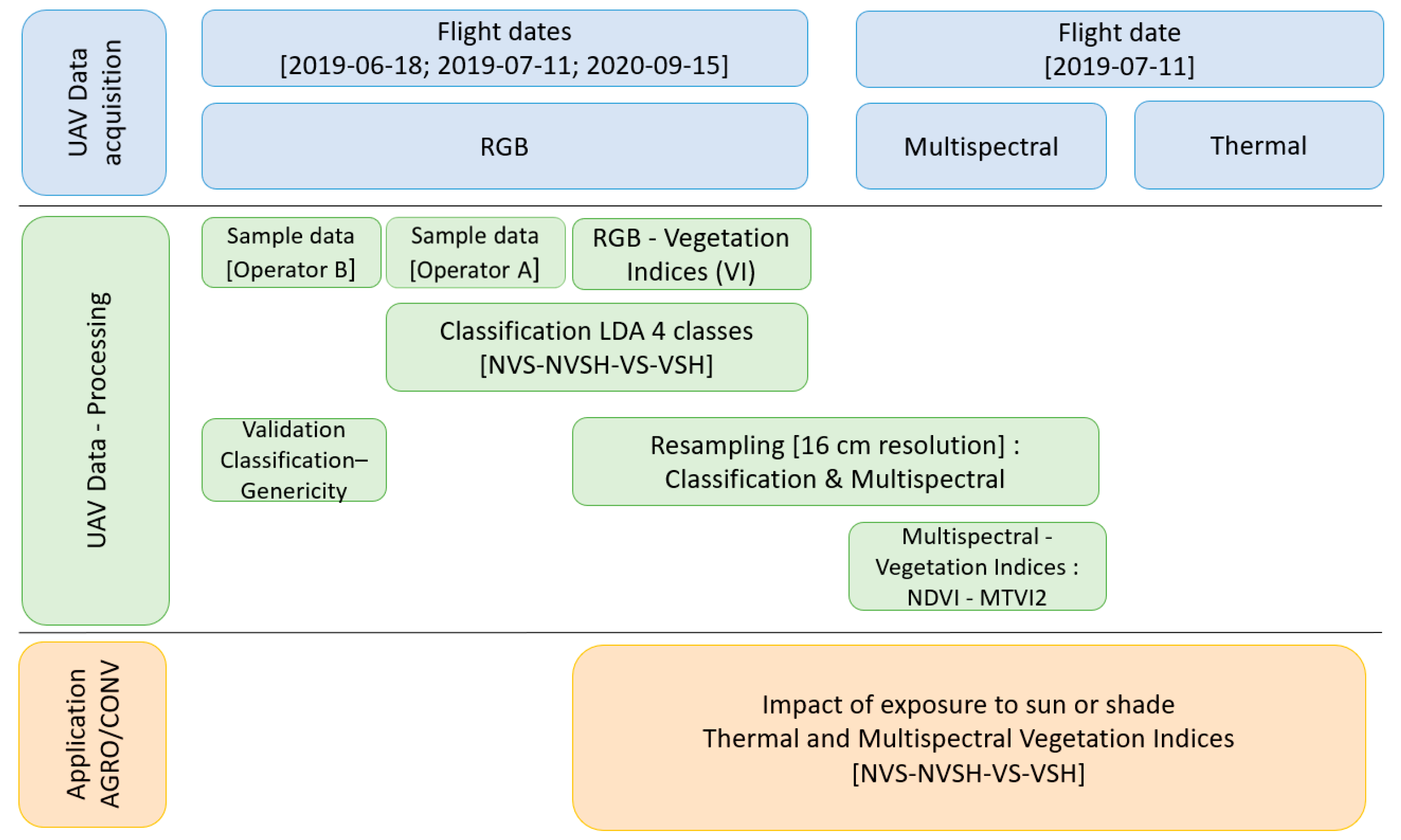
2.3.1. UAV Data

The UAV images were collected under clear sky conditions using a Sensefly eBee Classic rear-propeller UAV equipped with a 20 million pixels natural colour (RGB) S.O.D.A. camera (SenseFly, Cheseaux-sur-Lausanne, Switzerland), a MultiSPEC 4C multispectral sensor (Airinov, Paris, France), and a Thermomap thermal sensor (SenseFly, Cheseaux-sur-Lausanne, Switzerland). The aircraft was guided by a flight plan and flew at an altitude of 120 m. It was stabilized by an inertial central unit and could obtain images with a spatial resolution of about 3 cm for the RGB images, about 13 cm for the MS images and 20 cm for the thermal images (Table 2). Since a flight lasted about 30 min, about 2 h elapsed between the RGB and thermal sensor flight. Images were acquired throughout the 2019 growing season, with the first acquisition in March 2018 and the last in September 2020. An ortho-rectified mosaic, with differential GPS centimeter calibration, was produced using Pix4D (Pix4D S.A., Prilly, Switzerland) from more than 300 shots, each measuring 6000 × 4000 pixels (65% linear and 70% lateral coverage). It covered a surface of about 60 ha located in the center of the concerned area and involved approximately 29,600 × 337,600 pixels. The images are precisely recalibrated by incorporating Ground Control Points, targets placed on the ground whose coordinates are measured using a differential GPS. The coordinates of these targets are recalculated in post-processing to improve their accuracy (GPS Pathfinder Office software 5.60). Moreover, for the multispec4C, before each flight, an automatic radiometric calibration is carried for each sensor.
Deployment of the present methodology was based on RGB imagery, which is supplied in digital counts. The other images were used for validation purposes. In the present work, RGB imagery has been chosen for its resolution. The 11th of July 2019 was chosen as a reference date for the study, as the ground cover includes crop residues, bare soil, and vegetation at various stages of development (Table 1).
The thermal images, in brightness temperature, contributed to the assessment of the impact of sunshine on the soil and vegetation. The reflectance MS images were used to calculate the NDVI and MTVI2 indices (Table 2).

2.3.2. Sample Data

Samples useful for detection were separated according to (i) their exposition to direct or indirect sunlight (sun and shade) and (ii) the type of ground cover. The samples were collected from the RGB image using photo interpretation. Given the accuracy of RGB images, the accuracy of DGPS (Differential Global Positioning System), the errors related to the orthorectification of UAV images, and the reality observed in the field or by the sensor, the collection of GPS points in situ was considered unfeasible [40]. The photo-interpreted data was used for identifying four classes: vegetation in the sun (VS), vegetation in the shade (VSH), no vegetation in the sun (NVS), and no vegetation in the shade (NVSH) (Figure 2). Indeed, the two types of ground cover present need to be discriminated in order to distinguish the areas that are in the sun and in the shade at nadir observation during the time of the RGB flight (Table 2).
In order to minimize any operator bias during photo interpretation, the data was collected by two separate operators. These data were distributed over the plot and included an unequal number of points since they depend on the class and the operator (Figure 2). During July, given the stage of vegetation development and the time of the flight (solar noon) (Table 1), the observation acquired by a remote sensing sensor at the nadir associated to shade was less present and in lower quantities.
The non-vegetated class is associated with bare soil on the CONV plot or to soil covered with crop residues on the AGRO plot. The shaded non-vegetated class (NVSH) represents soil/residue areas shaded by the ground (due to its irregularities) or by spontaneous vegetation. The vegetation class corresponds to maize crops but also to areas occupied by weeds. In both classes, the term “sun” represents areas that visually benefit from direct sunlight in each RGB image. In contrast, the word “shade” in the RGB images indicates the visual impact of indirect solar radiation. Shaded vegetation is a more complicated class to identify, especially when the canopy’s development stage only consists of a few leaves and when the leaves are only a few centimeters wide (Table 1).

3. Method for Automatic Detection of Shaded and Sunlit Surfaces

The process used to analyse the impact of solar irradiation on temperature and vegetation indices for pixels with and without vegetation is illustrated in the synoptic diagram in Figure 3.

3.1. Vegetation Indices (VI)

In order to improve the detection of sunshine according to the type of land cover, several of the most commonly used vegetation indices were derived from the original spectral bands (R, G, B) (Table 3). The colour index for vegetation (CIVE), the vegetation difference in the visible band index (VDVI), the excess green indices (ExG and ExGR) and the combined indices (COM [8,41]) are all designed to identify and extract the presence of green vegetation. The modified green-red vegetation index (MGRVI) and the red-green-blue index (RGBVI) are considered as phenology indicators and can contribute to biomass estimation. The Red-Green Ratio Index (RGRI) is designed to estimate the chlorophyll content. For soil, Escadafal et al. [3] demonstrated how soils can be characterised by indices relating to the brightness of colour: these include colour saturation (SI), intensity (SCI, HUE) or brightness (BI). The Vegetation Colour Index reveals the difference between red and green and is used for separating the two types of cover (presence and absence of vegetation).
In addition, the four monitored land cover types were distinguished by testing the three R-G-B spectral bands as well as sixteen VIs (Table 3), i.e., in total nineteen variables.
Vegetation indices were calculated from multispectral images, the normalised difference vegetation index (NDVI) and the modified triangular vegetation index (MTVI2). These allow for photosynthetic activity to be assessed. The MTVI2 is used to compensate for the saturation of the NDVI [53]. These two indices were used for characterising each land cover class’s spatial dynamics and separability.

3.2. Choice of Predictor Variables and Detection of the Four Land Cover Classes

The nineteen predictor variables (known as primitives) were not all used for detecting land cover classes, so the most discriminating ones were selected according to a correctness rate (CR) (Equation (5)). The chosen method was based on a multivariate approach and used linear predictive discriminant analysis (LDA). This is one of the oldest discrimination techniques and was proposed by Fischer in 1936 [54]. Its main principle is to optimise separability between classes in order to identify them in the best possible way. The contribution of each primitive was determined according to its contribution to the separation of the four classes. The selection of the most relevant primitives took into account all the samples produced by the two operators (Figure 2). In this manner, each sampled pixel was associated to nineteen values corresponding to its spectral response in the R, G and B bands and to the 16 VIs. The most relevant primitives for obtaining the optimal separability of the selected classes were retained. The prediction was top-down, incorporating all the primitives that were successively removed. Significance was calculated by cross-validation on ten tests, by randomly splitting the samples. When the maximum value of the chosen criterion was less than the defined “improvement”, the corresponding variable was excluded from the classification.
This classification was carried out by calculating a model based on the samples. It consists of an estimation of the statistical characteristics in the LDA equation and is based on data from a single operator. Therefore, for each type of land cover of a sample, the model identified the position of the point representing the barycentre of each class in the multivariate space of primitives. The resulting factor axes, linear discriminants (LD), were straight lines along which the points were projected.
The prediction model was then applied in order to generate the final classification image so that each pixel in the final image would be assigned to one of the four groups. For each pixel, the classification used the minimum distance to the barycentre of each class. In this manner, each pixel was assigned to the group with the closest barycentre. Data from the second operator served to validate the classification image using Overall Accuracy (OA) (Equation (1)), Kappa [55] and F-measure (Equation (4)). The robustness of the proposed methodology for the separation of sun shade from canopy was assessed by generating a model for the 3 study dates (Table 2). The issue of the genericity of a single model that would be applicable to other dates in the development stage and also to another crop was also addressed based on the model created for a single date (Section 5).
For the classification images, the samples separated into two sets by operators A and B (Figure 2) were never mixed. Operator bias was ruled out by testing them in turn for model training or for validation of the classification image. A change in operator led to variations in Overall Accuracy (OA) performance by (+/−0.005). All samples from both operators were stored (Figure 2). The data from operator A was used to create the model, while the data from operator B was used for validation purposes, and represented the reference class. As the proportions of each class were not identical for each operator, a random draw of 200 points per class was tested for the creation of the model on 11 July 2019 and repeated 10 times. This threshold of 200 represents the minimum quantity of samples collected by operator A for the VSH class (Figure 2). Variations in OA were negligible (−0.01), suggesting that the results were not sample-dependent, and all samples were used.
The classification was validated based on the number of pixels in the reference class using a confusion matrix [56]. The performance indices used for overall relevance were evaluated according to the rates of True Positives (Tp), True Negatives (Tn), False Positives (Fp) and False Negatives (Fn). The false positive rate quantifies pixels from the reference class that were wrongly positioned in other classes. The false negative rate quantifies pixels which were placed in a given class but should belong to another. The kappa determines the relative difference between the observed and random proportions of agreement [55].
The Overall Accuracy (OA) provides the ratio between the correctly sorted elements and the total number of examined elements. (Equation (1)). The kappa coefficient is not an index of precision, since it does not measure overall agreement, but agreement beyond chance [57]. Nevertheless, it is combined here with the OA to assess the overall performance of the classification.
O A = T p + T n ( T p + T n + F p + F n )
Precision (P) and Recall (R) (Equations (2) and (3)) correspond, respectively, to the percentage of pixels from the reference class that were assigned to the correct group, and the percentage of correctly assigned pixels relative to the total number of pixels in the class.
P = T p T p + F n
R = T p T p + F p
These parameters contribute to infer the F-measure (FM) used in this study (Equation (4)), which corresponds to the harmonic mean of precision and recall [58]:
F M e a s u r e = 2 × P × R P + R
This score has the advantage of falling sharply when one of the parameters (P or R) is low and of rising when both are similar and high.
The Correctness Rate (CR) is reported as a percentage. It refers to the probability of achieving a correct detection and is calculated by subtracting the false positive (Fp) and false negative (Fn) rates from 1 (Equation (5)).
C R = ( 1 F p F n ) × 100 %
This rate can be used for measuring the relative importance of the different primitives when creating the classification model.

3.3. Re-Sampling of Classification Images

The classification image, generated from RGB image data at 3 cm spatial resolution, was re-sampled at a 16 cm resolution (cubic interpolation) so it could be used with temperature images (16 cm) and NDVI and MTVI2 indices (12 cm) (Table 3). For the brightness temperature and NDVI and MTVI2 images, 75% pure pixels were retained (Figure 4a) for the study. Indeed, a pixel purity threshold of less than 100% had to be set in order to retain the four land cover classes. Shade classes that had a limited number of contiguous pixels were affected. Figure 4b. illustrates the loss of information associated with the change in resolution.
The loss of 8.7 ha on the 20 ha plot (i.e., 43.7%) mainly affected shaded areas where contiguous pixels at 3 cm were scarce. For example, the shaded vegetation class, which represented 10% (1.65 ha) of the area of the plot at 3 cm resolution, was reduced to 0.4% (0.07 ha) after re-sampling at 16 cm resolution, while the shaded bare ground lost around 12% of its area (Figure 4b). For the 16 cm pixels that did not meet the fixed criteria, the proportions of the four classes at 3 cm pixels lay significantly below 75% (median VSH = 11%, median NVSH = 21%, VS = 45%, NVS = 13%). Since 43.7% of the ground was made up of pure patches that measured less than 16 cm on each side, the estimation of temperature was hardly relevant for 3 cm sized pixels that were mostly isolated.
The MS images, after re-sampling with a cubic interpolation method, could visually be perfectly superimposed on the RGB images and the classification. To reduce the effects of geometric distortion with thermal image, due to a different flight configuration, the later was cut into thumbnails according to a 100 × 100 m grid, and each thumbnail was georeferenced to the RGB image (Figure 5) using cubic interpolation and a polynomial transformation of degree three. For each thumbnail, a total of about 10 points were used to reset the image, thus allowing the classification to be used on thermal images.
The NDVI and MTVI2 indices were calculated on the re-sampled image.

4. Results and Analysis

The performance of the classification model was first presented at the native resolution of the RGB images (3 cm) for application to both CONV and AGRO plots and then by evaluating the model for each plot. The second part of the results involves the application of the classification to images that were re-sampled to 16 cm for brightness temperature and NDVI and MTVI2 indices. The separability of the four classes was analysed according to the objects’ responses to sun and shade. The differences in systemic functioning between the CONV and AGRO plots and the effects of exposure to sun or shade were consequently highlighted.

4.1. Evaluation of the Classification Model Performed on the RGB Image at 3 cm Resolution

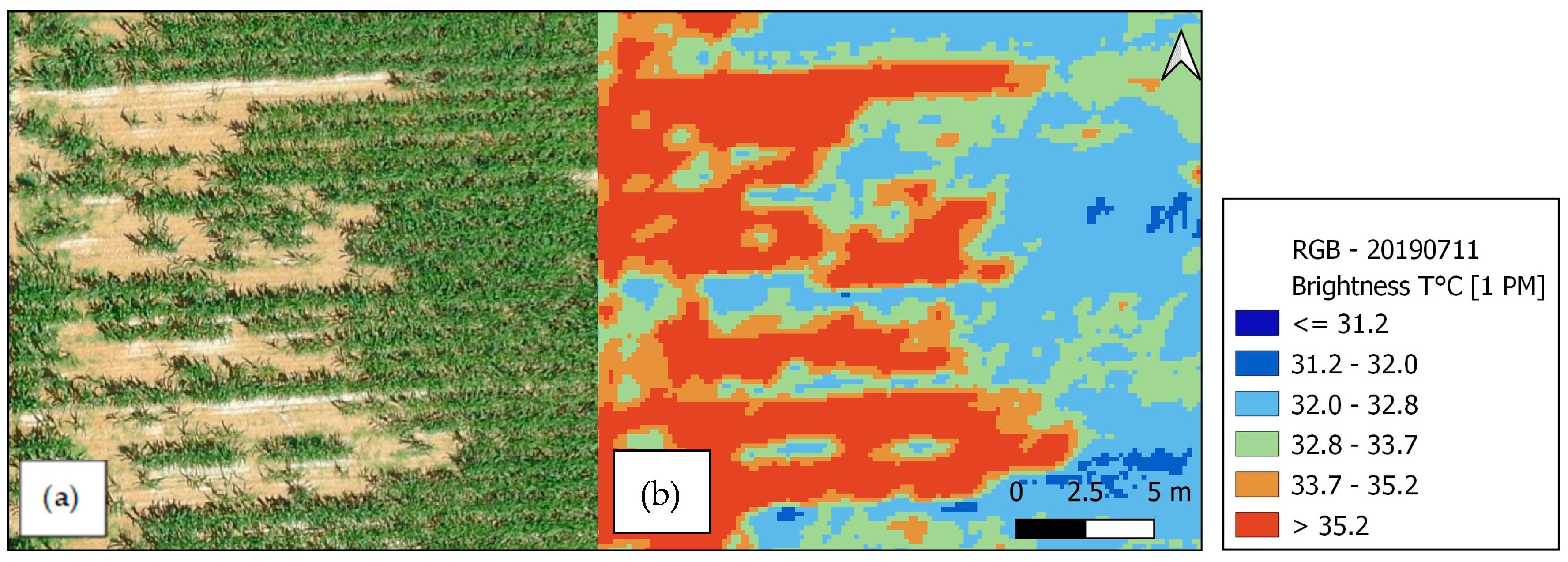
4.1.1. Application to the Entire Site during the Vegetation Season (11 July 2019)

The CR accuracy rate, estimated during the classification prediction step, was 0.978 with the nineteen primitives. With the COM2 index alone, this rate reaches 0.90 and then increased as the other primitives were progressively added. With twelve primitives, the CR reached 0.982, then stabilized or even lightly decreased when the remaining seven primitives were progressively added. Guerrero et al. 2012 [41] simultaneously selected greenness indices (Table 3) in order to improve the distinction between irrigated maize and weeds during segmentation. They highlighted the benefit of this combination, which reduced the mixing rate between vegetation surfaces and soils even subsequent to water input. The use of COM2 as the most discriminating primitive was therefore found to be in line with this reasoning.
The classification image produced from a model based on nineteen primitives gives an AO of 0.95 and a Kappa of 0.91. When the twelve most discriminating variables were used for creating the final classification, the OA increased by 0.004 (Figure 6) and the Kappa by 0.01, reaching 0.92. To select the primitives, ten random draws were made in order to avoid a potential sample effect. The twelve most frequent VIs and spectral bands were retained. These twelve primitives were the 3 RGB bands and the 9 VIs: Red, Green, Blue, SCI, GLI, SI, CIVE, COM2, MGRVI, EXGr, ExG, Color Index are defined in Table 3.
Figure 6 illustrates how each class of land cover could be distinguished by its own reflectance behavior, although some overlap occurred, particularly between VS and VSH on the first two linear discriminants. Furthermore, a hundred and twenty one VSH pixels of VSH were classified as VS (p = 0.89, F-measure = 0.57). This was related to the creation itself of the samples used and to the difficulty in visual detection of the shadows of the leaves, especially when the latter were about 3 cm wide. Vegetation observed in the shade at the nadir only represented 10% of the total surface area, in comparison with 61% of sunlit vegetation (Figure 4). The vegetation (V) and non-vegetation (NV) classes remained very distinct, with only eleven VSH pixels that were incorrectly classified as NVSH. The non-vegetated surface, whether in the sun or shade, was very well detected, with F-measures of 0.99 and 0.97 for NVS and NVSH, respectively.

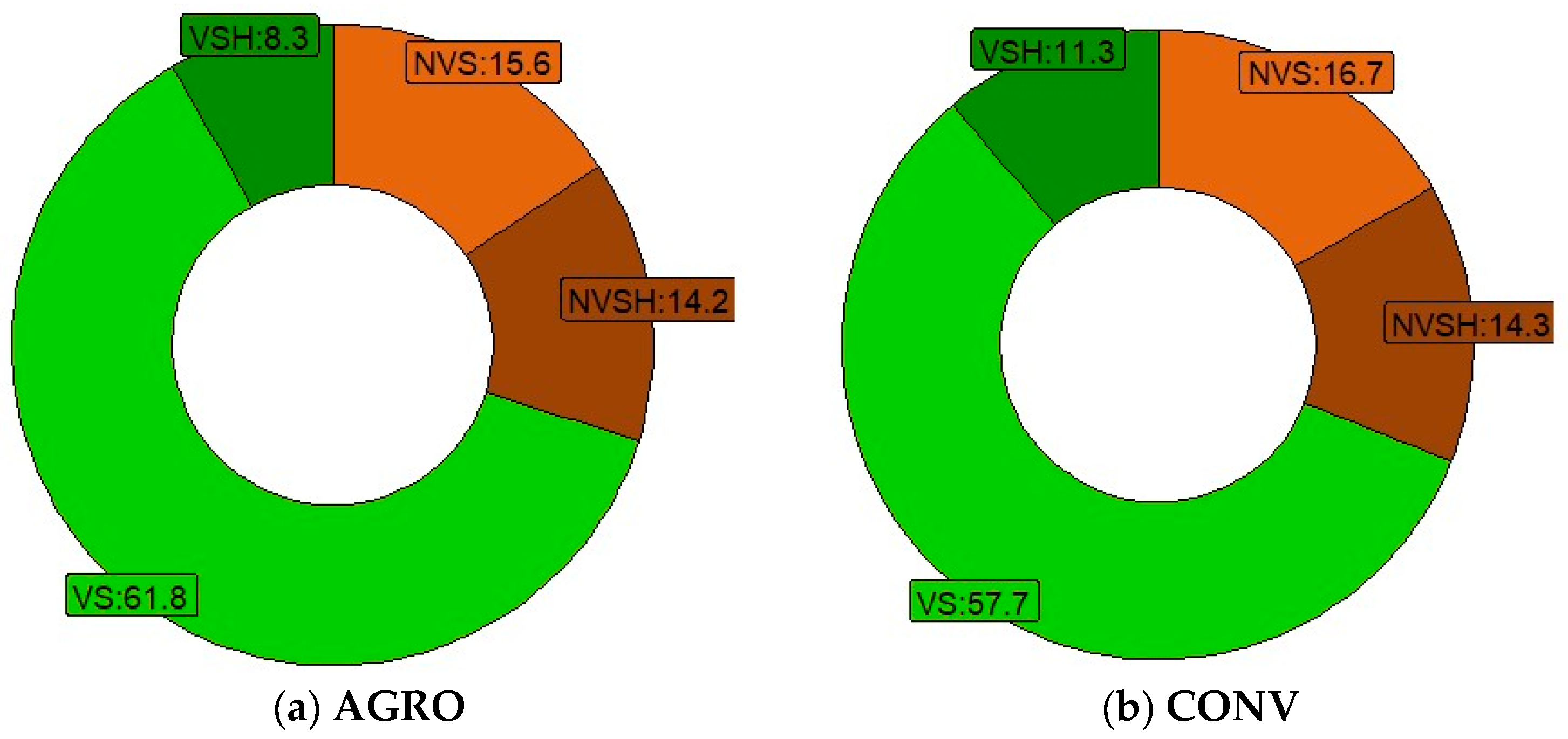
4.1.2. Separation of Results by Crop Type: AGRO/CONV (for the 11 July 2019)

The separate classification validation for each plot produced a Kappa of 0.86 and 0.98 and an OA of 0.90 and. 0.99 for the AGRO and CONV plots, respectively. The lower values observed for the AGRO plot could be due to a more important mixing of elements (V and NV) in the shade and sun. The overall distribution of the four types of land cover on both plots (Figure 7) suggested that, under similar observation conditions, the differences in the proportions of NV and V remained minor. Indeed, the overall area associated to vegetation (V) or soil (NV) varied by +/−1% (VAGRO = 70%, VCONV = 69%, NVAGRO = 30%, NVCONV = 31%).
Nevertheless, the proportion of the VS area for AGRO was 4% higher than that of the VS for CONV. Moreover, the shade/sun distribution illustrates that, overall, the shaded area detected by the RGB sensor at the nadir for AGRO was smaller (−3%). This is due to a narrower inter-row spacing, i.e., 0.40 m for AGRO compared with 0.80 m for CONV (Table 1). However, even though there may have been confusion in the classification, these were probably related, on the one hand, to the presence of low height vegetation (regrowth) within the residues of the AGRO plot and, on the other hand, to the structure of the canopy based on its layout (inter-row distance, inter-plant distance) and its geometry (nine leaves vs. flowering) which was different in this plot.

4.2. Application of Classification to Temperature and Vegetation Index Images at 16 cm Resolution

In order to assess the relevance of the mask produced during the classification of the July image, this mask was applied, after re-sampling at 16 cm spatial resolution, to the temperature images collected at 12:49 p.m. and to the two vegetation indices, NDVI and MTVI2. Indeed, the thermal behavior of the study area exhibited inter- and intra-plot variability, which would be worth analysing by class according to the effects of sunlight.

4.2.1. Overall Results for the Entire Study Site

For the whole study area, the comparison of temperature values at 12:49 p.m. and of the various indices for each land-use class (vertical line = mean) pointed out that the temperature of the NV class was generally higher than that of the V class (mean + ~3°). In addition, sunlit areas (whether NV or V) were warmer than the respective (NV or V) shaded areas for the median of the distribution (mean + ~1°).
For the V classes, according to the sunlight, the global difference in temperature was negligible (~0.4 °C) and virtually non-existent for the NDVI and MTVI2 vegetation indices (~0.04). However, the differences were significant for the NV classes (Figure 8). Non-vegetated areas (Figure 8) represented the less representative classes, with only 14.8% (2.45 ha) for NVS and 14.5% (2.40 ha) for NVSH. The mask separated these two latter classes according to both the temperature and vegetation index distributions. The median soil temperature in the sun (NVS) was 2.4 °C higher than in the shade (NVSH). The two vegetation indices differed by 26.6% (in relative percentage) for NDVI (median) and by 12.2% for MTVI2 (Figure 8) between NVS and NVSH. This result is discussed in further detail below. Concerning the vegetation, differences were negligible (<1%) independently of the vegetation index, as was expected.

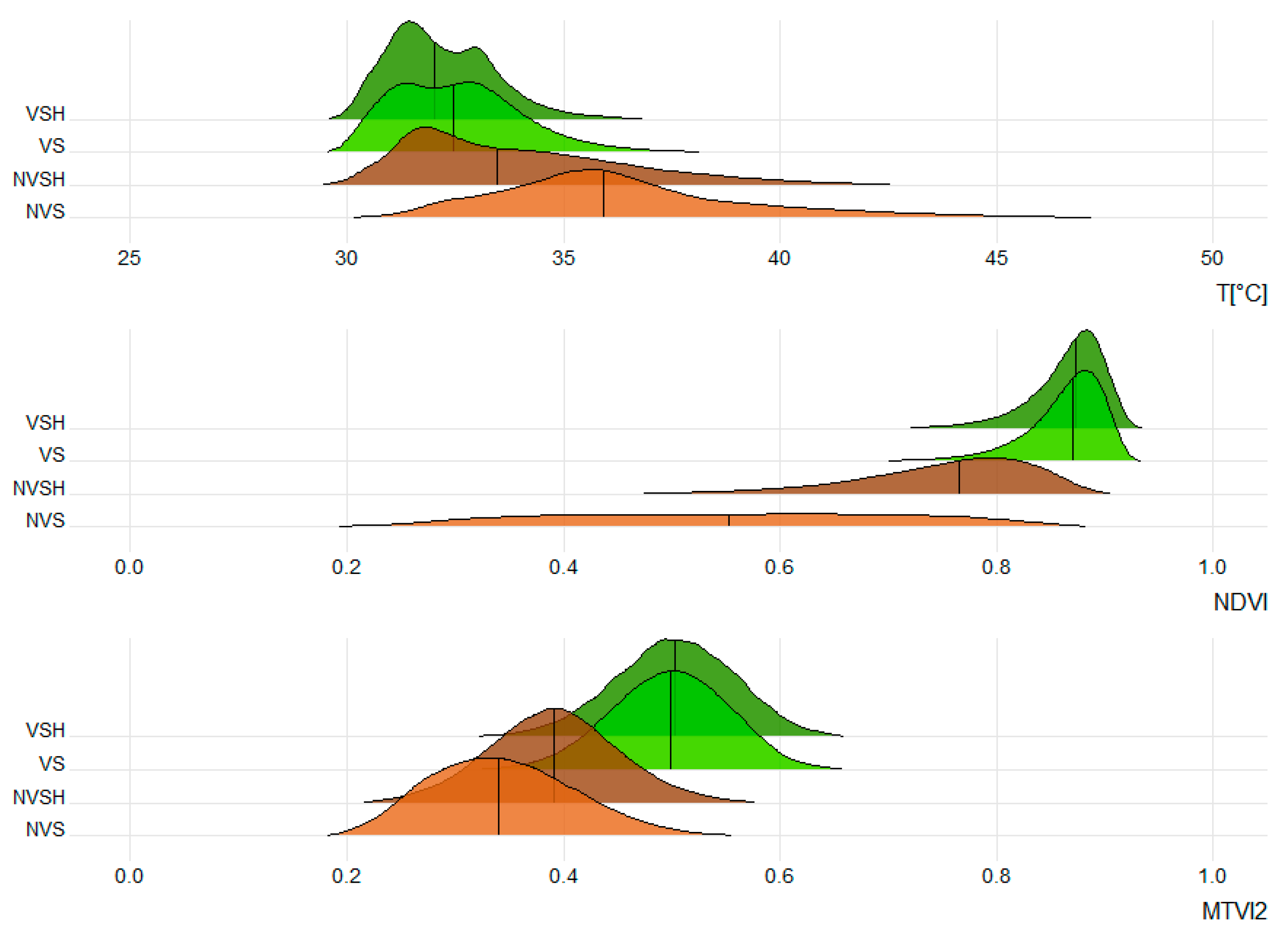
4.2.2. Separation of Temperature Results for AGRO and CONV

In order to refine the analysis, results were provided for each CONV and AGRO plot (Figure 9). In general, 72.5% of the data from the AGRO plot could not be used, compared with 71.3% for the CONV plot. Indeed, this arises because the number of classification patches (land use unit of a single class), when all classes are considered, is higher for the AGRO plot (nAGRO = 1,971,682) than for the CONV plot (nCONV = 1,752,135). Therefore, it was more strongly affected by the re-sampling at 16 cm due to the fewer amount of pure pixels.
In terms of temperature, the AGRO plot was warmer than the CONV plot, +2 °C for the vegetation and +2.9 °C for the NV surfaces (Figure 9 and Figure 10). The higher soil temperature on AGRO was related to the presence of crop residues. These results are corroborated by measurements of air temperature in the canopy, using temperature micro-sensors (Thermohygro iButtons, Analog Devices, Wilmington, MA, USA). The average temperature difference around solar noon between the 15 June 2019 and the 30 September 2019 was 2.5 °C (with an R2 = 0.88). The causes of these differences have not been detailed here, since they have been observed elsewhere and are the subject of other studies (BAG’AGES project) studies. These observations highlight the different thermo-hydric behavior patterns between both plots.
Concerning the shaded vegetation (VSH) at the CONV plot, there is a significant pixel density on the right hand side of the temperature distribution (Figure 10). This indicates the presence of zones called heat islands where temperatures are higher than the rest. Figure 10 illustrates this particular feature for areas where the cover is less dense. The increase in density of points relates to small areas of vegetation situated inside larger areas of bare ground (Figure 9). These heat islands may also derive from a VSH detection issue in these specific locations. However, visually, according to their location, these low density vegetation areas are more likely to cause locally higher temperatures through radiative effects (higher ground reflection and less shading under a scarcer canopy).
In order to assess the relevance of the mask produced, focus was put on the results obtained for non-vegetated areas with shading effects (NVS and NVSH). These areas are indeed minority classes where the total percentage represented 30% and only 8.5%, respectively, before and after re-sampling (Figure 4).
For the NV areas, the differences in temperature between shade and sun were 2.5 °C at the AGRO plot and 2.2 °C at the CONV plot. The spatial variability of the temperature (distributions ranged between the 1st and 9th decile) was nevertheless significantly different between both plots. Ranges were 33.5 < T°NVSH < 39.2 for the AGRO plot and 30.8 < T°NVSH < 34.1 for the CONV plot. The diversity of the surface soil of the AGRO plot was made up of a mixture of residues, non-residues, dry soil, damp soil and herbaceous plants, which, depending on their proportions, contribute to this temperature range at decametric resolution (Figure 10). Moreover, a difference between the more marked NVS and NVSH at the CONV plot could be observed on the NDVI. This will be discussed in Section 4.2.3.
Regardless of crop management, vegetated areas with similar crop densities and development presented very slight temperature differences between sunlit vegetation in the sun and shaded vegetation.
Similar tests were performed using the 3:10 pm temperature image. Considering the time elapsed between the acquisition of the RGB image and the second thermal flight (~5 h) as well as the displacement of shadows, the classes were assembled independently of their solar irradiance at 10:28 am (NVS and NVSH, and VS and VSH) so as to finally obtain only 2 classes: NV and V. The temperature difference between CONV and AGRO plots measured at 12:49 pm was observed again at 3:10 pm for both the NV and V classes.

4.2.3. Separation of AGRO and CONV Results for Vegetation Indices

For Vegetation Indices, the differences between NVS and NVSH were more pronounced for NDVI and the CONV plot. Apart from confirming the separability of the classes using the obtained classification, this result raises the question of the origin and impact of this difference. Figure 11 compares fifty non-contiguous points (twenty-five points on the AGRO plot followed by twenty-five points on the CONV plot) of NDVI and MTVI2 for the four land cover classes.
The effect of shading by vegetation on the ground affected vegetation indices to a significant extent for NDVI and to a lesser extent for MTVI2 at the CONV plot. Indeed, the NDVI of NVS on the CONV plot varied between 0.23 and 0.65 (range of distributions between the 1st and last decile) with an average of 0.43 compared to 0.70 at the AGRO plot. This could be explained by higher spectral values in the red on the bare ground than on the residue-covered ground, resulting in a higher NDVI at the AGRO plot than at the CONV plot. Considering the NVSH, the NDVI of both plots were close, with an average NDVI of 0.75 for the AGRO plot and 0.72 for the CONV plot. Non-vegetated areas in the shade (bare ground and residues) presented an NDVI comparable to that of a grassy area or even a crop. This could be explained by the fact that the shadow on non-vegetated surfaces was actually the shadow of the vegetation, which itself absorbs most of the red radiation. This was clearly demonstrated with these decametric resolution data, but raised the issue of soil detection for shaded areas at decametric resolution.
The MTVI2 amplitude was less significant for the NVS class (0.24 < MTVI2 < 0.45); the average MTVI2 at the CONV plot was 0.31 and 0.36 at the AGRO plot, and the differences between shade and sun were minor.
The effects of shading on the vegetation cover were slight, with similar variations of MTVI2 and NDVI on VS and VSH respectively, and on both plots. These result from red radiation being rather absorbed by the vegetation than by the soil (Figure 11B,C).
Regarding the impact of shade on NDVI, the use of MTVI2 relative to the NDVI should therefore be preferred when calculating a stress indicator (TVDI type, [59]) combining surface temperature and NDVI vegetation index with very high-resolution UAV data or on areas with shaded ground.

5. Summary and Discussion

Two cropping systems were monitored: the first under conventional agriculture (CONV) and the second under conservation agriculture (AGRO). Both plots grew maize in 2019. 16 vegetation indices from R, G and B bands and 2 Vegetation Indices from multispectral data at centimetric resolution (UAV images) were evaluated as primitive for separating four classes: vegetation in the shade (VSH), vegetation in the sun (VS), non-vegetation in the shade (NVSH), non-vegetation in the sun (NVS).
A classification model was developed for three specific dates (11 July 2019, 18 June 2019 and 15 September 2020) associated with different stages of crop development. The twelve most discriminating primitives were retained for the final classification.
The classification was aggregated at 16 cm so it could be applied to images of brightness temperature and vegetation indices with lower resolution. The time difference between the acquisition of RGB and thermal images had a limited effect on the shading zones due to the east-west orientation of the rows in the monitored plots and to the solar angle of the study site. Class separability was then verified for temperature, NDVI and MTVI2. According to the results, when an entire plot was considered, vegetated areas were less affected by shading than non-vegetated areas: i.e., sunlit elements showed +3 °C for soil and +1 °C for vegetation.
The classification was applied separately to CONV and AGRO, resulting in an OA of 0.99 and 0.90, respectively, and a kappa of 0.98 and 0.86, respectively, for the 11 July 2019, even though the percentage distribution of the four classes was virtually equivalent. The weaker separation performance of all four classes on the AGRO plot could be explained by higher mixing rates, which may be due, in particular, to crop residues lying on the ground.
In addition, AGRO vegetation was 2 °C warmer than CONV vegetation, while no-vegetation was 2.9 °C warmer, that were corroborated by microclimatic monitoring measurements. At the CONV plot, certain areas had a poor growth rate, and the vegetation in the shade (VHS) therefore presented heat islands with temperatures about 2 °C higher.
Spatial temperature variability was higher for AGRO: (33.5 < T°NVSH AGRO < 39.2 and 30.8 < T°NVSH CONV < 34.1). This difference is related to the diversity of the AGRO plot surface soil and to the mulch effect of crop residues that limit surface soil evaporation.
The NDVI increased, on one hand, due to the shade of the vegetation and on the other hand due to the presence of soil residues (on the AGRO plot). Each of these two factors can reduce red reflectance and thus increase the NDVI: mean NDVINVS CONV = 0.36, NDVINVS AGRO = 0.70 and mean NDVINVSH > 0.70.
A first point of discussion concerns the robustness and genericity of the methodology which were assessed for the three dates. A summary table of the performances is presented in Table 4. For each date, the twelve major primitives were calculated and samples were generated using the same methods as for July 2019. The samples were also separated in the same way. To create the model for the 18 June 2019, 200 sample points were generated for shadows in non-vegetated areas and 250 points for shadows in vegetated areas. During classification, the reflectance of the classes, whether vegetated or not, overlapped with their shadows in the first two linear discriminants. If the OA was 0.96 (Kappa = 0.93), the confusion matrix highlighted confusion at the level of shaded areas without vegetation and sunlit vegetation (PNVSH = 0.59, FM NVSH = 0.80). The detection of shade at this stage in the development of the canopy, or the creation of samples and the classification process, implies there is a limitation. This was not apparent in the results, but only in visualizing the classified image. For the AGRO plot, the leaves were at a leaf development stage of 4 out of 5, with a height of about 30 cm (Table 1). The vegetation was hardly visible on the RGB image at 3 cm spatial resolution. The plot was covered with residues and there was virtually no shade. For the CONV plot, the maize had an average of 8 leaves out of 9 and reached about 60 cm high. The shadow of the leaves on the ground was visible, but given the geometry and spacing of the plants, there was virtually no shadow on the vegetation.
Considering the image of 15 September 2020, there were two stages of vegetation on the AGRO plot: the southern part was covered with maize in an early senescent stage while the northern part was covered with maize residues (Table 1). On the CONV plot, soya plants were at a senescent phase. The vegetation class on either CONV or AGRO, independent of the crop type (maize or soya) or stage, was assimilated to the corresponding VS/VSH class (according to its illumination) without taking senescence into account.
The September model was generated with 550 points of senescent vegetation in sunlight and 740 points of full vegetation in sunlight. The reflectance of the VS samples differed from the other classes irrespective of the stage or crop. This was illustrated in the confusion matrix, with an F-measure of 0.99 for VS and 0.89 for VSH and very little confusion. The NV classes were subject to more mixing between classes however, without reaching the level of confusion observed at the other dates.
In order to test the genericity of the classification model for the July, when maize was in full development, the model was evaluated on the other available image dates (Table 4). In this way, other phenological stages and stand densities could be covered, with differences in plant architecture. Moreover, tests could be performed on other types of crops, i.e., in the present case soya crops (Table 1).
For the June 2019 image, acquired at the onset of the maize growing season, the 11 July 2019 model proposed a kappa of 0.75 (OA = 0.87), with results revealing mixtures between vegetation and shaded ground. As for the 15 September 2020 image acquired at the end of the season in the following year, when soybeans were grown on the CONV plot, this model predicted a large amount of mixing between vegetation in the senescent phase and green vegetation, with a kappa of 0.55 (OA = 0.68). This mixing could be easily explained by the spectral similarity between the residual and vegetation pixels. With only four types of land cover classes (VS, VSH, NVS and NVSH) and no specific adaptations, such as considering the spectral values of different crop types during the growing season when building the model, it would be difficult to use a single model, particularly at the end of the growing season. In such cases, the authors recommend the number of classes should be increased (e.g., the distinction between senescent and non-senescent vegetation) by adapting it to the general context and by re-generating a new classification model. In the case a single model is used, the definition of the classes would have to take into account all the phenological stages.
Another point of discussion concerns the way in which shadows are considered when using UAV images in actual studies. They are, for example, sampled to monitor water stress or the health of nectarine and peach orchards [60]. Recent articles, on the contrary, have used classification methods to eliminate them in the context of monitoring abiotic stress (frost) [19], water stress [61] or water monitoring to control yield and wine quality [62]. These current methods consist of detecting shadows and filtering them by thresholding or modelling [60]. The shadow class has not been studied as such because of its more or less rapid temporal evolution depending on the architecture of the canopy and the orientation of the rows. To our knowledge, this is an original feature of this study which contributes in particular to a better description of canopy temperature distributions over the different classes with decametric resolutions. This is of interest for 3D modelling of DART radiative transfer [39,63] for fine-resolution simulation of brightness temperature. A better description of sub-pixel temperature is currently a challenge for the TRISHNA space mission [64] which aims at the fine monitoring of microclimatic variability within ecosystems.
Moreover, the effect of vegetation shading also affects NDVI, which increases. These values could then be compared with NDVI values calculated for grassy areas at a resolution of 10m resolution. The MTVI2 was not significantly impacted by these factors, thus it would play a better role than NDVI as a VI to be employed in drought indicators such as TVDI-type drought indicators at these decametric scale resolutions. The use and limitations of NDVI, including its increase due to shading effects, should therefore be considered, at lower resolutions, particularly for detection in orchards and vineyards, which involve inter-row grass cover.

6. Conclusions

With the aim to investigate the details of the behavior of agricultural canopies, four land cover classes were separated: vegetation in the shade (VSH), vegetation in the sun (VS), non-vegetation in the shade (NVSH), non-vegetation in the sun (NVS).
The methodology is based on vegetation indices (VI) from multispectral UAV images at decametric resolution and R, G, B bands with UAV images at 3 cm resolution combined in order to conduct a linear discriminant analysis (LDA). The separability of the four classes was validated with good accuracy.
This study contributes to the evaluation of agricultural practices such as agroecology and their microclimatic effects within vegetation cover.
Differences in vegetation and non-vegetation temperature distributions between two contiguous maize plots in conventional agriculture (CONV) vs. conservation agriculture (AGRO) have then been highlighted associated to different thermo-hydric functioning.
The study is a prerequisite for better informing and constraining physical modelling at the soil-plant-atmosphere interface as well as the rate of land cover.
It also provides insights into the estimation and use of nadir shadow proportions in aggregated pixels (from 3 cm towards lower resolution) for photosynthesis modeling, by considering the proportion of sunlit and shaded areas [65].
Vegetation shading effects on NDVI also suggests discussing its choice for calculating stress indicators or for use in modeling.
Regarding the re-sampling methodology for classification, the authors next propose to retain the proportions of each mixing pole (VS, NVS, VSH, NVSH) within each aggregated pixel in order to spatially invert their characteristics (temperature maps of each pole, NDVI and/or MTVI2 maps of each pole, etc.). The method would then be applied to decametric remote sensing images (i.e., Sentinel 2) in order to feed modelling approaches that distinguish the functioning of vegetation growth in the shade and the sun.

Author Contributions

Conceptualization and methology, C.M.-S., S.Q., V.B., L.L., N.P. and B.C.; software, C.M.-S. and S.Q.; validation, C.M.-S., S.Q., V.B., N.B. and B.C.; resources, H.B.; data curation, C.M.-S., S.Q. and H.B.; writing—original draft preparation, C.M.-S., S.Q., V.B., N.P. and B.C. All authors have read and agreed to the published version of the manuscript.

Funding

This research received no external funding.

Data Availability Statement

The data presented in this study are available on request from the corresponding author.

Acknowledgments

Data acquisition at FR-Estampes are mainly funded by the Adour-Garonne water agency (BAG’AGES project) and the Institut National des Sciences de l’Univers (INSU) through the OSR SW observatory (https://osr.cesbio.cnrs.fr/, (accessed on 30 march 2024)). Facilities and staff are funded and supported by the Observatory Midi-Pyrenean, the University Paul Sabatier of Toulouse 3, CNRS (Centre National de la Recherche Scientifique), CNES (Centre National d’Etudes Spatiales), INRAE (Institut National de Recherche en Agronomie et Environnement), and IRD (Institut de Recherche pour le Développement). Our special thanks go to Rousseau and to Abadie, farmers, for accommodating our measurement devices in their respective fields.

Conflicts of Interest

The authors declare no conflicts of interest.

References

  1. Gates, D.M.; Keegan, H.J.; Schleter, J.C.; Weidner, V.R. Spectral Properties of Plants. Appl. Opt. 1965, 4, 11. [Google Scholar] [CrossRef]
  2. Hatfield, J.L.; Gitelson, A.A.; Schepers, J.S.; Walthall, C.L. Application of Spectral Remote Sensing for Agronomic Decisions. Agron. J. 2008, 100, S-117–S-131. [Google Scholar] [CrossRef]
  3. Escadafal, R. Remote Sensing of Soil Color: Principles and Applications. Remote Sens. Rev. 1993, 7, 261–279. [Google Scholar] [CrossRef]
  4. Bannari, A.; Pacheco, A.; Staenz, K.; McNairn, H.; Omari, K. Estimating and Mapping Crop Residues Cover on Agricultural Lands Using Hyperspectral and IKONOS Data. Remote Sens. Environ. 2006, 104, 447–459. [Google Scholar] [CrossRef]
  5. Jordan, C.F. Derivation of Leaf-Area Index from Quality of Light on the Forest Floor. Ecology 1969, 50, 663–666. [Google Scholar] [CrossRef]
  6. Hatfield, J.L.; Prueger, J.H.; Sauer, T.J.; Dold, C.; O’Brien, P.; Wacha, K. Applications of Vegetative Indices from Remote Sensing to Agriculture: Past and Future. Inventions 2019, 4, 71. [Google Scholar] [CrossRef]
  7. Hatfield, J.L.; Prueger, J.H. Value of Using Different Vegetative Indices to Quantify Agricultural Crop Characteristics at Different Growth Stages under Varying Management Practices. Remote Sens. 2010, 2, 562–578. [Google Scholar] [CrossRef]
  8. Guijarro, M.; Pajares, G.; Riomoros, I.; Herrera, P.J.; Burgos-Artizzu, X.P.; Ribeiro, A. Automatic Segmentation of Relevant Textures in Agricultural Images. Comput. Electron. Agric. 2011, 75, 75–83. [Google Scholar] [CrossRef]
  9. Lee, M.-K.; Golzarian, M.R.; Kim, I. A New Color Index for Vegetation Segmentation and Classification. Precis. Agric. 2021, 22, 179–204. [Google Scholar] [CrossRef]
  10. Xue, J.; Su, B. Significant Remote Sensing Vegetation Indices: A Review of Developments and Applications. J. Sens. 2017, 2017, 1353691. [Google Scholar] [CrossRef]
  11. Rouse, J.W., Jr.; Haas, R.H.; Schell, J.A.; Deering, D.W. Monitoring Vegetation Systems in the Great Plains with Erts. In NASA Special Publication; NASA: Washington, DC, USA, 1974; Volume 351, p. 309. [Google Scholar]
  12. Tucker, C.J. Red and Photographic Infrared Linear Combinations for Monitoring Vegetation. Remote Sens. Environ. 1979, 8, 127–150. [Google Scholar] [CrossRef]
  13. Hamuda, E.; Glavin, M.; Jones, E. A Survey of Image Processing Techniques for Plant Extraction and Segmentation in the Field. Comput. Electron. Agric. 2016, 125, 184–199. [Google Scholar] [CrossRef]
  14. Hunt, E.R.; Doraiswamy, P.C.; McMurtrey, J.E.; Daughtry, C.S.T.; Perry, E.M.; Akhmedov, B. A Visible Band Index for Remote Sensing Leaf Chlorophyll Content at the Canopy Scale. Int. J. Appl. Earth Obs. Geoinf. 2012, 21, 103–112. [Google Scholar] [CrossRef]
  15. Giovos, R.; Tassopoulos, D.; Kalivas, D.; Lougkos, N.; Priovolou, A. Remote Sensing Vegetation Indices in Viticulture: A Critical Review. Agriculture 2021, 11, 457. [Google Scholar] [CrossRef]
  16. Jantzi, H.; Marais-Sicre, C.; Maire, E.; Barcet, H.; Guillerme, S. Diachronic Mapping of Invasive Plants Using Airborne RGB Imagery in a Central Pyrenees Landscape (South-West France). In Proceedings of the IECAG 2021, Basel, Switzerland, 11 May 2021; p. 51. [Google Scholar]
  17. Ayamga, M.; Akaba, S.; Nyaaba, A.A. Multifaceted Applicability of Drones: A Review. Technol. Forecast Soc. Change 2021, 167, 120677. [Google Scholar] [CrossRef]
  18. Kumar, A.; Shreeshan, S.; Tejasri, N.; Rajalakshmi, P.; Guo, W.; Naik, B.; Marathi, B.; Desai, U.B. Identification of Water-Stressed Area in Maize Crop Using Uav Based Remote Sensing. In Proceedings of the 2020 IEEE India Geoscience and Remote Sensing Symposium (InGARSS), Ahmedabad, India, 1–4 December 2020; pp. 146–149. [Google Scholar]
  19. Goswami, J.; Sharma, V.; Chaudhury, B.U.; Raju, P.L.N. Rapid identification of abiotic stress (frost) in in-filed maize crop using UAV remote sensing. Int. Arch. Photogramm. Remote Sens. Spat. Inf. Sci. 2019, 42, 467–471. [Google Scholar] [CrossRef]
  20. Singh, A.P.; Yerudkar, A.; Mariani, V.; Iannelli, L.; Glielmo, L. A Bibliometric Review of the Use of Unmanned Aerial Vehicles in Precision Agriculture and Precision Viticulture for Sensing Applications. Remote Sens. 2022, 14, 1604. [Google Scholar] [CrossRef]
  21. Matese, A.; Di Gennaro, S. Practical Applications of a Multisensor UAV Platform Based on Multispectral, Thermal and RGB High Resolution Images in Precision Viticulture. Agriculture 2018, 8, 116. [Google Scholar] [CrossRef]
  22. Moller, M.; Alchanatis, V.; Cohen, Y.; Meron, M.; Tsipris, J.; Naor, A.; Ostrovsky, V.; Sprintsin, M.; Cohen, S. Use of Thermal and Visible Imagery for Estimating Crop Water Status of Irrigated Grapevine. J. Exp. Bot. 2006, 58, 827–838. [Google Scholar] [CrossRef]
  23. Gontia, N.K.; Tiwari, K.N. Development of Crop Water Stress Index of Wheat Crop for Scheduling Irrigation Using Infrared Thermometry. Agric. Water Manag. 2008, 95, 1144–1152. [Google Scholar] [CrossRef]
  24. Jones, H.G.; Serraj, R.; Loveys, B.R.; Xiong, L.; Wheaton, A.; Price, A.H. Thermal Infrared Imaging of Crop Canopies for the Remote Diagnosis and Quantification of Plant Responses to Water Stress in the Field. Funct. Plant Biol. 2009, 36, 978. [Google Scholar] [CrossRef] [PubMed]
  25. Alchanatis, V.; Cohen, Y.; Cohen, S.; Moller, M.; Sprinstin, M.; Meron, M.; Tsipris, J.; Saranga, Y.; Sela, E. Evaluation of Different Approaches for Estimating and Mapping Crop Water Status in Cotton with Thermal Imaging. Precis. Agric. 2010, 11, 27–41. [Google Scholar] [CrossRef]
  26. Romano, G.; Zia, S.; Spreer, W.; Sanchez, C.; Cairns, J.; Araus, J.L.; Müller, J. Use of Thermography for High Throughput Phenotyping of Tropical Maize Adaptation in Water Stress. Comput. Electron. Agric. 2011, 79, 67–74. [Google Scholar] [CrossRef]
  27. Feng, L.; Chen, S.; Zhang, C.; Zhang, Y.; He, Y. A Comprehensive Review on Recent Applications of Unmanned Aerial Vehicle Remote Sensing with Various Sensors for High-Throughput Plant Phenotyping. Comput. Electron. Agric. 2021, 182, 106033. [Google Scholar] [CrossRef]
  28. Sagan, V.; Maimaitijiang, M.; Sidike, P.; Eblimit, K.; Peterson, K.T.; Hartling, S.; Esposito, F.; Khanal, K.; Newcomb, M.; Pauli, D.; et al. UAV-Based High Resolution Thermal Imaging for Vegetation Monitoring, and Plant Phenotyping Using ICI 8640 P, FLIR Vue Pro R 640, and Thermomap Cameras. Remote Sens. 2019, 11, 330. [Google Scholar] [CrossRef]
  29. Maimaitijiang, M.; Ghulam, A.; Sidike, P.; Hartling, S.; Maimaitiyiming, M.; Peterson, K.; Shavers, E.; Fishman, J.; Peterson, J.; Kadam, S.; et al. Unmanned Aerial System (UAS)-Based Phenotyping of Soybean Using Multi-Sensor Data Fusion and Extreme Learning Machine. ISPRS J. Photogramm. Remote Sens. 2017, 134, 43–58. [Google Scholar] [CrossRef]
  30. Wang, T.; Chandra, A.; Jung, J.; Chang, A. UAV Remote Sensing Based Estimation of Green Cover during Turfgrass Establishment. Comput. Electron. Agric. 2022, 194, 106721. [Google Scholar] [CrossRef]
  31. Avola, G.; Filippo, S.; Gennaro, D.; Cantini, C.; Riggi, E.; Muratore, F.; Tornambè, C.; Matese, A. Remote Sensing Communication Remotely Sensed Vegetation Indices to Discriminate Field-Grown Olive Cultivars. Remote Sens. 2019, 11, 1242. [Google Scholar] [CrossRef]
  32. Grillakis, M.G.; Doupis, G.; Kapetanakis, E.; Goumenaki, E. Future Shifts in the Phenology of Table Grapes on Crete under a Warming Climate. Agric. Meteorol. 2022, 318, 108915. [Google Scholar] [CrossRef]
  33. Olsson, L.; Barbosa, H.; Bhadwal, S.; Cowie, A.; Delusca, K.; Flores-Renteria, D.; Hermans, K.; Jobbagy, E.; Kurz, W.; Li, D.; et al. Land Degradation. In Climate Change and Land; Cambridge University Press: Cambridge, UK, 2022; pp. 345–436. [Google Scholar]
  34. Mbow, C.; Rosenzweig, C.; Barioni, L.G.; Benton, T.G.; Herrero, M.; Krishnapillai, M.; Liwenga, E.; Pradhan, P.; RiveraFerre, M.G.; Sapkota, T.; et al. Food Security. In Climate Change and Land; Cambridge University Press: Cambridge, UK, 2022; pp. 437–550. [Google Scholar]
  35. Altieri, M.A. Agroecology: The Scientific Basis of Alternative Agriculture; Intermediate Publications: London, UK, 1987. [Google Scholar]
  36. Baize, D.; Girard, M.C. Référentiel Pédologique; Association Française pour L’étude du Sol: Versailles, France, 2008. [Google Scholar]
  37. Alletto, L.; Cueff, S.; Bréchemier, J.; Lachaussée, M.; Derrouch, D.; Page, A.; Gleizes, B.; Perrin, P.; Bustillo, V. Physical Properties of Soils under Conservation Agriculture: A Multi-Site Experiment on Five Soil Types in South-Western France. Geoderma 2022, 428, 116228. [Google Scholar] [CrossRef]
  38. Breil, N.L.; Lamaze, T.; Bustillo, V.; Marcato-Romain, C.-E.; Coudert, B.; Queguiner, S.; Jarosz-Pellé, N. Combined Impact of No-Tillage and Cover Crops on Soil Carbon Stocks and Fluxes in Maize Crops. Soil Tillage Res. 2023, 233, 105782. [Google Scholar] [CrossRef]
  39. Boitard, P.; Coudert, B.; Lauret, N.; Queguiner, S.; Marais-Sicre, C.; Regaieg, O.; Wang, Y.; Gastellu-Etchegorry, J.-P. Calibration of DART 3D Model with UAV and Sentinel-2 for Studying the Radiative Budget of Conventional and Agro-Ecological Maize Fields. Remote Sens. Appl. 2023, 32, 101079. [Google Scholar] [CrossRef]
  40. La Salandra, M.; Colacicco, R.; Dellino, P.; Capolongo, D. An Effective Approach for Automatic River Features Extraction Using High-Resolution UAV Imagery. Drones 2023, 7, 70. [Google Scholar] [CrossRef]
  41. Guerrero, J.M.; Pajares, G.; Montalvo, M.; Romeo, J.; Guijarro, M. Support Vector Machines for Crop/Weeds Identification in Maize Fields. Expert Syst. Appl. 2012, 39, 11149–11155. [Google Scholar] [CrossRef]
  42. Richardsons, A.J.; Wiegand, A. Distinguishing Vegetation from Soil Background Information. Photogramm. Eng. Remote Sens. 1977, 43, 1541–1552. [Google Scholar]
  43. Mathieu, R.; Pouget, M.; Cervelle, B.; Escadafal, R. Relationships between Satellite-Based Radiometric Indices Simulated Using Laboratory Reflectance Data and Typic Soil Color of an Arid Environment. Remote Sens. Environ. 1998, 66, 17–28. [Google Scholar] [CrossRef]
  44. Louhaichi, M.; Borman, M.M.; Johnson, D.E. Spatially Located Platform and Aerial Photography for Documentation of Grazing Impacts on Wheat. Geocarto Int. 2001, 16, 65–70. [Google Scholar] [CrossRef]
  45. Gitelson, A.A.; Stark, R.; Grits, U.; Rundquist, D.; Kaufman, Y.; Derry, D. Vegetation and Soil Lines in Visible Spectral Space: A Concept and Technique for Remote Estimation of Vegetation Fraction. Int. J. Remote Sens. 2002, 23, 2537–2562. [Google Scholar] [CrossRef]
  46. Zarco-Tejada, P.J.; Berjón, A.; López-Lozano, R.; Miller, J.R.; Martín, P.; Cachorro, V.; González, M.R.; De Frutos, A. Assessing Vineyard Condition with Hyperspectral Indices: Leaf and Canopy Reflectance Simulation in a Row-Structured Discontinuous Canopy. Remote Sens. Environ. 2005, 99, 271–287. [Google Scholar] [CrossRef]
  47. Kataoka, T.; Kaneko, T.; Okamoto, H.; Hata, S. Crop Growth Estimation System Using Machine Vision. In Proceedings of the 2003 IEEE/ASME International Conference on Advanced Intelligent Mechatronics (AIM 2003), Kobe, Japan, 20–24 July 2003; pp. b1079–b1083. [Google Scholar]
  48. Gamon, J.A.; Surfus, J.S. Assessing Leaf Pigment Content and Activity with a Reflectometer. New Phytol. 1999, 143, 105–117. [Google Scholar] [CrossRef]
  49. Bendig, J.; Yu, K.; Aasen, H.; Bolten, A.; Bennertz, S.; Broscheit, J.; Gnyp, M.L.; Bareth, G. Combining UAV-Based Plant Height from Crop Surface Models, Visible, and near Infrared Vegetation Indices for Biomass Monitoring in Barley. Int. J. Appl. Earth Obs. Geoinf. 2015, 39, 79–87. [Google Scholar] [CrossRef]
  50. Woebbecke, D.M.; Meyer, G.E.; Von Bargen, K.; Mortensen, D.A. Color Indices for Weed Identification Under Various Soil, Residue, and Lighting Conditions. Trans. ASAE 1995, 38, 259–269. [Google Scholar] [CrossRef]
  51. Meyer, G.E.; Neto, J.C. Verification of Color Vegetation Indices for Automated Crop Imaging Applications. Comput. Electron. Agric. 2008, 63, 282–293. [Google Scholar] [CrossRef]
  52. Eitel, J.U.H.; Long, D.S.; Gessler, P.E.; Smith, A.M.S. Using In-situ Measurements to Evaluate the New RapidEyeTMsatellite Series for Prediction of Wheat Nitrogen Status. Int. J. Remote Sens. 2007, 28, 4183–4190. [Google Scholar] [CrossRef]
  53. Hatfield, J.L.; Asrar, G.; Kanemasu, E.T. Intercepted Photosynthetically Active Radiation Estimated by Spectral Reflectance. Remote Sens. Environ. 1984, 14, 65–75. [Google Scholar] [CrossRef]
  54. Chiang, L.H.; Russell, E.L.; Braatz, R.D. Fault Detection and Diagnosis in Industrial Systems. Meas. Sci. Technol. 2001, 12, 1745. [Google Scholar] [CrossRef]
  55. Cohen, J. A Coefficient of Agreement for Nominal Scales. Educ. Psychol. Meas. 1960, 20, 37–46. [Google Scholar] [CrossRef]
  56. Congalton, R.G. A Review of Assessing the Accuracy of Classifications of Remotely Sensed Data. Remote Sens. Environ. 1991, 37, 35–46. [Google Scholar] [CrossRef]
  57. Foody, G.M. Explaining the Unsuitability of the Kappa Coefficient in the Assessment and Comparison of the Accuracy of Thematic Maps Obtained by Image Classification. Remote Sens Environ. 2020, 239, 111630. [Google Scholar] [CrossRef]
  58. Powers David, M.W. Evaluation: From Precision, Recall and F-Measure to ROC, Informedness, Markedness and Correlation. J. Mach. Learn. Technol. 2011, 2, 37–63. [Google Scholar]
  59. Sandholt, I.; Rasmussen, K.; Andersen, J. A Simple Interpretation of the Surface Temperature/Vegetation Index Space for Assessment of Surface Moisture Status. Remote Sens. Environ. 2002, 79, 213–224. [Google Scholar] [CrossRef]
  60. Park, S.; Ryu, D.; Fuentes, S.; Chung, H.; Hernández-Montes, E.; O’Connell, M. Adaptive Estimation of Crop Water Stress in Nectarine and Peach Orchards Using High-Resolution Imagery from an Unmanned Aerial Vehicle (UAV). Remote Sens. 2017, 9, 828. [Google Scholar] [CrossRef]
  61. Poblete, T.; Ortega-Farías, S.; Ryu, D. Automatic Coregistration Algorithm to Remove Canopy Shaded Pixels in UAV-Borne Thermal Images to Improve the Estimation of Crop Water Stress Index of a Drip-Irrigated Cabernet Sauvignon Vineyard. Sensors 2018, 18, 397. [Google Scholar] [CrossRef]
  62. Sepúlveda-Reyes, D.; Ingram, B.; Bardeen, M.; Zúñiga, M.; Ortega-Farías, S.; Poblete-Echeverría, C. Selecting Canopy Zones and Thresholding Approaches to Assess Grapevine Water Status by Using Aerial and Ground-Based Thermal Imaging. Remote Sens. 2016, 8, 822. [Google Scholar] [CrossRef]
  63. Regaieg, O.; Yin, T.; Malenovský, Z.; Cook, B.D.; Morton, D.C.; Gastellu-Etchegorry, J.-P. Assessing Impacts of Canopy 3D Structure on Chlorophyll Fluorescence Radiance and Radiative Budget of Deciduous Forest Stands Using DART. Remote Sens Environ. 2021, 265, 112673. [Google Scholar] [CrossRef]
  64. Lagouarde, J.-P.; Bhattacharya, B.K.; Crébassol, P.; Gamet, P.; Adlakha, D.; Murthy, C.S.; Singh, S.K.; Mishra, M.; Nigam, R.; Raju, P.V.; et al. Indo-French high-resolution thermal infrared space mission for Earth natural resources assessment and monitoring–Concept and definition of TRISHNA. Int. Arch. Photogramm. Remote Sens. Spat. Inf. Sci. 2019, 42, 403–407. [Google Scholar] [CrossRef]
  65. Norman, J.M.; Kustas, W.P.; Humes, K.S. Source Approach for Estimating Soil and Vegetation Energy Fluxes in Observations of Directional Radiometric Surface Temperature. Agric. For. Meteorol. 1995, 77, 263–293. [Google Scholar] [CrossRef]
Figure 1. The study site, represented with a Lambert-93 projection, with altitudes (m) on a Google satellite image.
Remotesensing 16 01436 g001
Figure 2. (a) Positioning of sample class types by operators (A or B) on the UAV image of the 11 July 2019. (b) Frequency of sampling points according to land use type and operator (11 July 2019).
Remotesensing 16 01436 g002
Figure 3. Synoptic diagram.
Remotesensing 16 01436 g003
Figure 4. From left to right: (a) RGB image of the 11 July 2019; Original classification at 3 cm resolution and Proportion [%] of the different classes of land cover before re-sampling. (b) Classification after re-sampling at 16 cm, Proportion [%] of the different classes of land cover that did not meet the 75% purity criterion, Proportion [%] of the different land cover classes of 75% purity and above.
Remotesensing 16 01436 g004
Figure 5. Map of the re-sampling of the 11 July 2019 thermal image.
Remotesensing 16 01436 g005
Figure 6. Classification performance measurements using the twelve primitives selected for the 11 July 2019 image and positioning of the samples on the first two linear discriminants (LD1 and LD2).
Remotesensing 16 01436 g006
Figure 7. Percentage distribution in 4 classes for each plot: NV, NVSH, VS, VSH, (a) AGRO plot, (b) CONV plot.
Remotesensing 16 01436 g007
Figure 8. Comparison of temperature values at 12:49 pm and various indices for each land-use class (NVS light brown, NVSH dark brown, VS light green, VSH dark green).
Remotesensing 16 01436 g008
Figure 9. (a) Part of UAV- RGB image from the 11 July 2019 (CONV plot), (b) Thermal UAV image of brightness temperature (CONV plot).
Remotesensing 16 01436 g009
Figure 10. Comparison of the temperature values at 12:49 p.m., of the indices and of the land use class (NVS light brown, NVSH dark brown, VS light green, VSH dark green) between both plots.
Remotesensing 16 01436 g010
Figure 11. Values of the NDVI (dotted line) and MTVI2 (solid line) indices for NVS, NVSH, VS, VSH classes—25 AGRO points followed by 25 CONV points.
Remotesensing 16 01436 g011
Table 1. Technical itinerary and phenological benchmarks for both AGRO and CONV plots.
Conservation Practice: AGRO PlotConventional Practice: CONV Plot
18 June 2019Crop residues (n − 1, weeds) & Corn emergence (4–5 leaf stage)
Inter-rows: 0.4 m/inter-feet: 0.25 m
Sprinkler irrigation: 105 mm
Corn (8–9 leaf stage)
Inter-rows: 0.8 m/inter-feet: 0.125 m
Sprinkler irrigation: 120 mm
11 July 2019Corn (8–9 leaf stage)Corn flowering
15 September 2020Two vegetation stages: North Corn senescence, South Late Flowering corn.Soybean senescence
Table 2. Technical characteristics and acquisition periods of the UAV imagery.
Flight DateStart Flight HourFlight Altitude [m]Resolution [m]
Multi Spectral2019-06-1812:57 PM1340.14
(multiSPEC4C sensor) G 550 nm -2019-07-1111:49 AM1150.12
R 660 nm—RE 735 nm—NIR 790 nm2020-09-1511:11 AM1340.14
Thermal (Thermomap sensor)T°1—2019-07-1112:49 PM850.16
7.2 & 13.5 nmT°2—2019-07-1103:10 PM850.16
RGB2019-06-1812:12 PM1230.03
(SODA senso)2019-07-1110:28 AM1150.03
R 450 nm—G 520 nm—B 660 nm2020-09-1510:35 AM1230.03
Table 3. Vegetation Indices (VI) used in the study (16 vegetation indices from R, G and B bands and 2 Vegetation Indices from multispectral data).
VIDescriptionEquationReference
BIBrightness Indexsqrt ((R^ + G2 + B2)/3)Richardson & Wiegand [42]
SCISoil Colour Index(R − G)/(R + G)Mathieu et al. [43]
GLIGreen Leaf Index(2 × G − R − B)/(2 × G + R + B)Louhaichi et al. [44]
HIHue index(2 × R − G − B)/(G − B)Escadafal [3]
SiSpectral Slope Saturation Index(R − B)/(R + B)Escadafal [3]
VARIVisible Atmospherically Resistant Index(G − R)/(G + R − B)Gitelson et al. [45]
HUEOverall Hue Indexarctan(2 × (B − G − R)/30.5(G − R))Escadafal [3]
BGIBlue green pigment indexB/GZarco-Tejada et al. [46]
CIVEColour Index of Vegetation Extraction(0.441 × R) − (0.881 × G) + (0.385 × B) + 18.78745Kataoka et al. [47]
COM2Combined Indices (COM2)(0.36 × E × G) + (0.47 × CIVE) + (0.17 × (G/(R0.667 × B0.333)))Guerrero et al. [42]
RGRI R/GGamon and Surfus [48]
MGRVIModified Green Red Vegetation Index(G2 − R2)/(G2 + R2)Bendig et al. [49]
RGBVIRed Green Blue Vegetation Index(G2 − R × B)/(G2 + R*B)Bendig et al. [49]
EXGExcess Green Index2 × G − R − BWoebbecke et al. [50]
EXGRExcess Green minus Red IndexExG − (1.4 × R − G)Meyer and Neto [51]
Colour IndexColour IndexR − G“Non-normalised index, no specific reference”
NDVINormalized Difference Vegetation IndexNIR − R/NIR + RTucker et al. [12]
MTVI2Modified Triangular Vegetation Index(1.5 × (1.2 × (NIR − R) − 2.5 × (G − R)))/sqrt((2 × NIR +1)2 − (6 × NIR − 5 × sqrt(G)) − 0.5)Eitel et al. [52]
Table 4. Robustness and genericity of the classification models.
Model11 July 2019 Model18 June 2019 Model15 September 2020 Model
Date OAKappaOAKappaOAKappa
11 July 20190.950.92xxxx
18 June 20190.870.750.960.93xx
15 September 20200.680.55xx0.960.94
Disclaimer/Publisher’s Note: The statements, opinions and data contained in all publications are solely those of the individual author(s) and contributor(s) and not of MDPI and/or the editor(s). MDPI and/or the editor(s) disclaim responsibility for any injury to people or property resulting from any ideas, methods, instructions or products referred to in the content.

