
A Spatiotemporally Constrained Interpolation Method for Missing Pixel Values in the Suomi-NPP VIIRS Monthly Composite Images: Taking Shanghai as an Example
 , and
, and
Abstract
:
1. Introduction
2. Study Area and Data
2.1. Study Area
2.2. Data
3. Methods
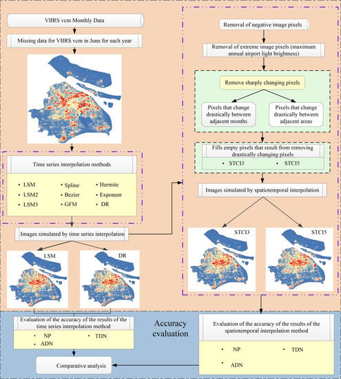
3.1. Research Ideas
3.2. Time Series Interpolation Method
3.3. Spatiotemporally Constrained Interpolation Method
3.3.1. Abnormal Pixel Removal
3.3.2. Time-Series Nighttime Light Relative Smoothness Feature Constraint
3.3.3. Constraints on the Relative Stability of the Urban Spatial Structure
3.3.4. Correction of Abnormal Pixels
3.4. Accuracy Evaluation
4. Results
4.1. Comparison of the Number of Abnormal Pixels
4.2. Comparison of Total Light Brightness
4.3. Comparison of Absolute Values of Differences
5. Discussion
6. Conclusions
- (1)
- Among the nine-time series interpolation methods used, the images simulated by the Spline method had the highest NP, the images simulated by the GFM method had the smallest NP, and the images simulated by the STCI3 method and the STCI5 method had no NP.
- (2)
- The TDN accuracy of the images simulated by the STCIM method was higher than that of the images simulated by the time series interpolation method, and the TDN accuracy of the images simulated by the STCI5 method was higher than that of the images simulated by the STCI3 method.
- (3)
- The number of pixels with an ADN between the light brightness of the image pixel simulated by the STCI5 method and the pixel light brightness of the corresponding position of the original image in the range of 0–1 was the largest. The number of pixels with an ADN between the light brightness of the image pixel simulated by the STCI3 method and the pixel light brightness of the corresponding position of the original image in the range of 0–5 was the largest. The accuracy of the STCIM method was higher than that of the time series interpolation method.
Author Contributions
Funding
Data Availability Statement
Acknowledgments
Conflicts of Interest
References
- Li, X.; Elvidge, C.; Zhou, Y.Y.; Cao, C.Y.; Warner, T. Remote sensing of night-time light. Int. J. Remote Sens. 2017, 38, 5855–5859. [Google Scholar] [CrossRef]
- Elvidge, C.D.; Baugh, K.E.; Kihn, E.A.; Kroehl, H.W.; Davis, E.R.; Davis, C.W. Relation between satellite observed visible-near infrared emissions, population, economic activity and electric power consumption. Int. J. Remote Sens. 1997, 18, 1373–1379. [Google Scholar] [CrossRef]
- Ma, T.; Xu, T.; Huang, L.; Zhou, A. A human settlement composite index (HSCI) derived from nighttime luminosity associated with imperviousness and vegetation indexes. Remote Sens. 2018, 10, 455. [Google Scholar] [CrossRef]
- Lu, D.; Wang, Y.H.; Yang, Q.Y.; Su, K.C.; Zhang, H.Z.; Li, Y.Q. Modeling Spatiotemporal Population Changes by Integrating DMSP-OLS and NPP-VIIRS Nighttime Light Data in Chongqing, China. Remote Sens. 2021, 13, 284. [Google Scholar] [CrossRef]
- Gu, Y.; Shao, Z.F.; Huang, X.; Cai, B.W. GDP Forecasting Model for China’s Provinces Using Nighttime Light Remote Sensing Data. Remote Sens. 2022, 14, 3671. [Google Scholar] [CrossRef]
- Doll, C.N.; Muller, J.P.; Morley, J.G. Mapping regional economic activity from night-time light satellite imagery. Ecol. Econ. 2006, 57, 75–92. [Google Scholar] [CrossRef]
- Chen, X.; Nordhaus, W.D. Using luminosity data as a proxy for economic statistics. Proc. Natl. Acad. Sci. USA 2011, 108, 8589–8594. [Google Scholar] [CrossRef]
- Li, X.; Ge, L.; Chen, X. Detecting Zimbabwe’s decadal economic decline using nighttime light imagery. Remote Sens. 2013, 5, 4551–4570. [Google Scholar] [CrossRef]
- Zhang, Q.; Seto, K.C. Mapping urbanization dynamics at regional and global scales using multi-temporal DMSP/OLS nighttime light data. Remote Sens. Environ. 2015, 115, 2320–2329. [Google Scholar] [CrossRef]
- Xu, T.; Ma, T.; Zhou, C.; Zhou, Y. Characterizing spatio-temporal dynamics of urbanization in China using time series of DMSP/OLS night light data. Remote Sens. 2014, 6, 7708–7731. [Google Scholar] [CrossRef]
- Chen, Z.Q.; Yu, B.L.; Song, W.; Liu, H.X.; Wu, Q.S.; Shi, K.F.; Wu, J.P. A New Approach for Detecting Urban Centers and Their Spatial Structure with Nighttime Light Remote Sensing. IEEE Trans. Geosci. Remote Sens. 2017, 55, 6305–6319. [Google Scholar] [CrossRef]
- Wang, R.; Wan, B.; Guo, Q.H.; Hu, M.S.; Zhou, S.P. Mapping Regional Urban Extent Using NPP-VIIRS DNB and MODIS NDVI Data. Remote Sens. 2017, 9, 862. [Google Scholar] [CrossRef]
- Jiang, L.G.; Liu, Y.; Wu, S.; Yang, C. Study on Urban Spatial Pattern Based on DMSP/OLS and NPP/VIIRS in Democratic People’s Republic of Korea. Remote Sens. 2021, 13, 4879. [Google Scholar] [CrossRef]
- Fan, J.F.; Ma, T.; Zhou, C.H.; Zhou, Y.K.; Xu, T. Comparative Estimation of Urban Development in China’s Cities Using Socioeconomic and DMSP/OLS Night Light Data. Remote Sens. 2014, 6, 7840–7856. [Google Scholar] [CrossRef]
- Fan, J.F.; He, H.X.; Hu, T.Y.; Zhang, P.; Yu, X.; Zhou, Y.K. Estimation of Landscape Pattern Changes in BRICS from 1992 to 2013 Using DMSP-OLS NTL Images. J. Indian Soc. Remote Sens. 2019, 7, 725–735. [Google Scholar] [CrossRef]
- Bagan, H.; Yamagata, Y. Analysis of urban growth and estimating population density using satellite images of nighttime lights and land-use and population data. GISci. Remote Sens. 2015, 52, 765–780. [Google Scholar] [CrossRef]
- Li, X.; Xu, H.M.; Chen, X.L.; Li, C. Potential of NPP-VIIRS nighttime light imagery for modeling the regional economy of China. Remote Sens. 2013, 5, 3057–3081. [Google Scholar] [CrossRef]
- Ma, J.J.; Guo, J.Y.; Ahmad, S.; Li, Z.Q.; Hong, J. Constructing a New Inter-Calibration Method for DMSP-OLS and NPP-VIIRS Nighttime Light. Remote Sens. 2020, 12, 937. [Google Scholar] [CrossRef]
- Li, X.; Zhou, Y.; Zhao, M.; Zhao, X. A harmonized global nighttime light dataset 1992–2018. Sci. Data 2020, 7, 168. [Google Scholar] [CrossRef]
- Yong, Z.W.; Li, K.; Xiong, J.N.; Cheng, W.M.; Wang, Z.G.; Sun, H.Z.; Ye, C.C. Integrating DMSP-OLS and NPP-VIIRS Nighttime Light Data to Evaluate Poverty in Southwestern China. Remote Sens. 2022, 14, 600. [Google Scholar] [CrossRef]
- Jing, X.; Shao, X.; Cao, C.; Fu, X.; Yan, L. Comparison between the Suomi-NPP Day-Night Band and DMSP-OLS for Correlating Socio-Economic Variables at the Provincial Level in China. Remote Sens. 2016, 8, 17. [Google Scholar] [CrossRef]
- Sutton, P.C. A scale-adjusted measure of “urban sprawl” using nighttime satellite imagery. Remote Sens. Environ. 2003, 86, 353–369. [Google Scholar] [CrossRef]
- Elvidge, C.D.; Baugh, K.E.; Anderson, S.J.; Sutton, P.C.; Ghosh, T. The night light development index (NLDI): A spatially explicit measure of human development from satellite data. Soc. Geogr. Discuss. 2012, 7, 23–35. [Google Scholar] [CrossRef]
- Ghosh, T.; Powell, R.L.; Elvidge, C.D.; Baugh, K.E.; Sutton, P.C.; Anderson, S. Shedding light on the global distribution of economic activity. Open Geogr. J. 2010, 3, 148–161. [Google Scholar] [CrossRef]
- Zhao, M.; Cheng, W.M.; Zhou, C.H.; Li, M.C.; Wang, N.; Liu, Q.Y. GDP Spatialization and Economic Differences in South China Based on NPP-VIIRS Nighttime Light Imagery. Remote Sens. 2017, 9, 673. [Google Scholar] [CrossRef]
- Mills, S.; Weiss, S.; Liang, C. VIIRS day/night band (DNB) stray light characterization and correction. In Proceedings of the Earth Observing Systems XVIII, San Diego, CA, USA, 25–29 August 2013; SPIE: Bellingham, WA, USA, 2013; Volume 8866, pp. 549–566. [Google Scholar] [CrossRef]
- Elvidge, C.D.; Zhizhin, M.; Ghosh, T.; Hsu, F.C.; Taneja, J. Annual time series of global VIIRS nighttime lights derived from monthly averages: 2012 to 2019. Remote Sens. 2021, 13, 922. [Google Scholar] [CrossRef]
- Zhao, N.; Hsu, F.C.; Cao, G.; Samson, E.L. Improving accuracy of economic estimations with VIIRS DNB image products. Int. J. Remote Sens. 2017, 38, 5899–5918. [Google Scholar] [CrossRef]
- Chen, M.L.; Cai, H.Y. Interpolation methods comparison of VIIRS/DNB nighttime light monthly composites: A case study of Beijing. Prog. Geogr. 2019, 38, 126–138. [Google Scholar] [CrossRef]
- Fan, J.F.; Zhang, P.; Chen, J.H.; Li, B.; Han, L.S.; Zhou, Y.K. Quantitative Estimation of Missing Value Interpolation Methods for Suomi-NPP VIIRS/DNB Nighttime Light Monthly Composite Images. IEEE Access. 2020, 8, 199266–199288. [Google Scholar] [CrossRef]
- Tian, S.C. The Least Squares Method of Statistical Principles and Applications in Agricultural Pilot Study. Math. Pract. Theory. 2015, 45, 124–133. Available online: https://kns.cnki.net/kcms/detail/detail.aspx?FileName=SSJS201504017&DbName=CJFQ2015 (accessed on 28 June 2022).
- Wang, B.B.; Li, H.J. Temperature Compensation of Piezoresistive Pressure Sensor Based on the Interpolation of Third Order Splines. Chin. J. Sens. Actuators 2015, 28, 1003–1007. [Google Scholar] [CrossRef]
- Li, X. Structure and Matlab Implementation of Cubic Spline Interpolation Endpoint Constraints. J. Shanghai Second. Polytech. Univ. 2012, 29, 319–323. [Google Scholar] [CrossRef]
- Shi, Y.; Jin, D.S. Electrocardiogram pattern recognition method combining bezier curve fitting. Comput. Eng. Des. 2013, 34, 1437–1441. [Google Scholar] [CrossRef]
- Deng, J.L. The main method of the intrinsic grey system. Syst. Eng. Theory Pract. 1986, 6, 60–65. [Google Scholar] [CrossRef]
- He, G. Forecast of regional logistics requirements and application of grey prediction model. J. Beijing Jiaotong Univ. 2008, 7, 33–37. [Google Scholar] [CrossRef]
- Wang, L.; Zhang, Q.; Huang, G.; Tian, J. GPS Satellite Clock Bias Prediction Based on Exponential Smoothing Method. Geomat. Inf. Sci. Wuhan Univ. 2017, 42, 995–1001. [Google Scholar] [CrossRef]
- Han, X. Shape-preserving piecewise rational interpolation with higher order continuity. Appl. Math. Comput. 2018, 337, 1–13. [Google Scholar] [CrossRef]
- Fritsch, F.N.; Carlson, R.E. Monotone piecewise cubic interpolation. SIAM J. Numer. Anal. 1980, 17, 238–246. [Google Scholar] [CrossRef]
- Shi, K.F.; Yu, B.L.; Huang, Y.X.; Hu, Y.J.; Yin, B.; Chen, Z.Q.; Chen, L.J.; Wu, J.P. Evaluating the ability of NPP-VIIRS nighttime light data to estimate the gross domestic product and the electric power consumption of China at multiple scales: A comparison with DMSP-OLS data. Remote Sens. 2014, 6, 1705–1724. [Google Scholar] [CrossRef]
- Ma, T.; Zhou, C.H.; Pei, T.; Haynie, S.; Fan, J.F. Responses of Suomi- NPP VIIRS- derived nighttime lights to socioeconomic activity in China’s cities. Remote Sens. Lett. 2014, 5, 165–174. [Google Scholar] [CrossRef]
- Zhao, N.; Zhou, Y.; Samson, E.L. Correcting Incompatible DN Values and Geometric Errors in Nighttime Lights Time-Series Images. IEEE Trans. Geosci. Remote Sens. 2014, 53, 2039–2049. [Google Scholar] [CrossRef]
- Cheng, G.; Li, Y.L.; Zhao, Z.Z.; Yang, J.; Lu, X.P.; Yuan, D.F. Spatiotemporal Interpolation Methods of NPP/VIIRS Sequence Images Considering Neighbor Relationships. Geomat. Inf. Sci. Wuhan Univ. 2022, 47, 252–260. [Google Scholar] [CrossRef]


| 2013 | 2014 | 2015 | 2018 | 2020 | 2021 | |
|---|---|---|---|---|---|---|
| PD | 215.1 | 196.4 | 211.3 | 391.8 | 314.9 | 339.3 |
| HQ | 263.7 | 212.5 | 235.9 | 435.2 | 585.1 | 438.5 |
| Threshold | 273.7 | 222.5 | 245.9 | 445.2 | 595.1 | 448.5 |
| 2013 | 2014 | 2015 | 2018 | 2020 | 2021 | |
|---|---|---|---|---|---|---|
| DR | 3 | 0 | 0 | 0 | 0 | 0 |
| Bezier | 16 | 0 | 3 | 5 | 1 | 0 |
| Exponent | 3 | 0 | 0 | 0 | 0 | 0 |
| GFM | 2 | 0 | 0 | 0 | 0 | 0 |
| LSM | 0 | 0 | 0 | 0 | 0 | 0 |
| LSM2 | 13 | 9 | 14 | 2 | 4 | 0 |
| LSM3 | 13 | 9 | 14 | 2 | 4 | 0 |
| Spline | 38 | 22 | 43 | 17 | 49 | 23 |
| Hermite | 4 | 0 | 1 | 0 | 3 | 0 |
| STCI3 | 0 | 0 | 0 | 0 | 0 | 0 |
| STCI5 | 0 | 0 | 0 | 0 | 0 | 0 |
Disclaimer/Publisher’s Note: The statements, opinions and data contained in all publications are solely those of the individual author(s) and contributor(s) and not of MDPI and/or the editor(s). MDPI and/or the editor(s) disclaim responsibility for any injury to people or property resulting from any ideas, methods, instructions or products referred to in the content. |
© 2023 by the authors. Licensee MDPI, Basel, Switzerland. This article is an open access article distributed under the terms and conditions of the Creative Commons Attribution (CC BY) license (https://creativecommons.org/licenses/by/4.0/).
Share and Cite
Liu, Q.; Fan, J.; Zuo, J.; Li, P.; Shen, Y.; Ren, Z.; Zhang, Y. A Spatiotemporally Constrained Interpolation Method for Missing Pixel Values in the Suomi-NPP VIIRS Monthly Composite Images: Taking Shanghai as an Example. Remote Sens. 2023, 15, 2480. https://0-doi-org.brum.beds.ac.uk/10.3390/rs15092480
Liu Q, Fan J, Zuo J, Li P, Shen Y, Ren Z, Zhang Y. A Spatiotemporally Constrained Interpolation Method for Missing Pixel Values in the Suomi-NPP VIIRS Monthly Composite Images: Taking Shanghai as an Example. Remote Sensing. 2023; 15(9):2480. https://0-doi-org.brum.beds.ac.uk/10.3390/rs15092480
Chicago/Turabian StyleLiu, Qingyun, Junfu Fan, Jiwei Zuo, Ping Li, Yunpeng Shen, Zhoupeng Ren, and Yi Zhang. 2023. "A Spatiotemporally Constrained Interpolation Method for Missing Pixel Values in the Suomi-NPP VIIRS Monthly Composite Images: Taking Shanghai as an Example" Remote Sensing 15, no. 9: 2480. https://0-doi-org.brum.beds.ac.uk/10.3390/rs15092480