
Leveraging CNNs for Panoramic Image Matching Based on Improved Cube Projection Model

Institute of Geospatial Information, The PLA Strategic Support Force Information Engineering University, Zhengzhou 450001, China
*
Author to whom correspondence should be addressed.
Remote Sens. 2023, 15(13), 3411; https://0-doi-org.brum.beds.ac.uk/10.3390/rs15133411
Submission received: 29 May 2023
/
Revised: 30 June 2023
/
Accepted: 3 July 2023
/
Published: 5 July 2023
(This article belongs to the Special Issue 3D City Modelling and Remote Sensing: Advances, Challenges, and New Technologies)
Abstract
:Three-dimensional (3D) scene reconstruction plays an important role in digital cities, virtual reality, and simultaneous localization and mapping (SLAM). In contrast to perspective images, a single panoramic image can contain the complete scene information because of the wide field of view. The extraction and matching of image feature points is a critical and difficult part of 3D scene reconstruction using panoramic images. We attempted to solve this problem using convolutional neural networks (CNNs). Compared with traditional feature extraction and matching algorithms, the SuperPoint (SP) and SuperGlue (SG) algorithms have advantages for handling images with distortions. However, the rich content of panoramic images leads to a significant disadvantage of these algorithms with regard to time loss. To address this problem, we introduce the Improved Cube Projection Model: First, the panoramic image is projected into split-frame perspective images with significant overlap in six directions. Second, the SP and SG algorithms are used to process the six split-frame images in parallel for feature extraction and matching. Finally, matching points are mapped back to the panoramic image through coordinate inverse mapping. Experimental results in multiple environments indicated that the algorithm can not only guarantee the number of feature points extracted and the accuracy of feature point extraction but can also significantly reduce the computation time compared to other commonly used algorithms.
1. Introduction
The panoramic image services provided by Google cover all seven continents, with images of areas inhabited by 98% of the world’s population [1,2]. Panoramic images have a wider perspective than typical perspective images, contain more comprehensive buildings and a stronger sense of reality, and have richer scene details [3]. Owing to the abundant resources and wide field of view (FOV), panoramic images have considerable advantages over perspective images in large-scale, three-dimensional (3D) scene reconstruction [4,5]. Three-dimensional scene reconstruction [6,7,8,9] has been comprehensively studied and applied to digital cities, virtual reality [10], and SLAM [11,12] because of its significant advantages in terms of model accuracy, realism, and ease of modeling. The key problem that needs to be solved to achieve 3D scene reconstruction is image matching [13,14,15]. Image matching is a core technology in digital photogrammetry [16] and computer vision and is mainly divided into two parts: feature extraction and feature matching. Only when robust and accurate image matching results are obtained can more complex work be performed with good results and continued in-depth research.
Owing to the characteristics of panoramic images, there are problems with image matching. As shown in Figure 1, most high-resolution panoramic images are obtained using combined lens cameras for various reasons, such as the imaging mechanism and perspective, resulting in significant nonlinear aberrations in different directions of the panoramic image [17]. This aberration is equivalent to adding a geometric transformation to a perspective image and increases with the distance from the center of the image. To solve the problem of panoramic image matching, numerous experiments have been performed. Most of the current panoramic image matching algorithms still rely on SIFT [18] because of its invariance to rotation, scale scaling, and grayscale changes. Therefore, the SIFT algorithm is robust for panoramic images with nonlinear distortions. However, the SIFT algorithm takes a lot of time to compute because of the scale space constructed. Additionally, the SURF [19] algorithm is an improvement on the SIFT algorithm, which greatly improves the computation speed of the SIFT algorithm and is more suitable for panoramic images with large amounts of data. The ORB [20] algorithm is faster than both the SIFT and ORB algorithms, but it is not rotation-invariant or scale-invariant because it is actually improved on the basis of the BRIEF [21] algorithm. The ASIFT [22] algorithm is improved on the basis of the SIFT algorithm. It is a fully affine-invariant algorithm, and SIFT only defines four parameters, while ASIFT defines six parameters, which is better for the adaptation of panoramic images. Most of these algorithms use distance-based methods, such as FLANN [23], for feature matching. However, the existence of obvious nonlinear distortion in a panoramic image leads to unsatisfactory results for distance-based matching methods between features. The CSIFT [24] algorithm, on the other hand, proposes SIFT-like descriptors while using kernel line constraints to improve the matching effect. These algorithms still apply the feature extraction and matching algorithms of perspective images directly or in an improved way to panoramic images and cannot adapt to the obvious nonlinear distortion of panoramic images.
In recent years, with the advancement of artificial intelligence, the convolutional neural network (CNN) [25,26], based on deep learning [27,28], has developed rapidly in the field of computer vision. For image feature extraction and matching, algorithms such as LIFT [29], SuperPoint [30], DELF [31], and D2-Net [32] have been proposed. With regard to feature extraction, the SP algorithm has the advantages of extracting a large number of features and fast computation and is widely used. With regard to feature matching, the traditional FLANN algorithm only considers the distance between features. The SuperGlue matching algorithm [33] surpasses the traditional FLANN algorithm by introducing an attentional graph neural network mechanism for both feature matching and mismatch rejection.
The Traditional Cube Projection Model [34] reprojects the panoramic image into six faces, but there is only one line connecting each face, resulting in poor continuity of the cube model, and each face corresponds to another for matching, and some faces may have a poor overlap rate and an unsatisfactory matching effect.
In this study, the deep learning method was applied to panoramic image matching, and the panoramic image obtained was used for experimental research. We present a practical approach for increasing the speed of deep feature extraction and matching and the number of features extracted through correction and sharing using the Improved Cube Projection Model. Our research provides a new perspective for panoramic image matching. The primary contributions of this study are summarized as follows:
- (1)
- The CNN is introduced to the field of panoramic image matching. We aimed to solve the problems of traditional algorithms, which do not have a strong generalization ability and have unsatisfactory applicability to panoramic images. Good results were obtained by matching the images using a CNN.
- (2)
- The Traditional Cube Projection Model was improved. To eliminate the characteristics of the discontinuity of the image in each split-frame image of the Traditional Cube Projection Model, the model was extended. Correction of the panoramic image distortion and accelerated matching were achieved using the Improved Cube Projection Model.
- (3)
- We propose a dense matching algorithm for panoramic images. It can accurately and efficiently achieve matching between such images, solving the challenge of matching panoramas with significant distortions.
The remainder of the paper is organized as follows: Section 2 presents the main process and principles of the proposed algorithm. Section 3 presents multiple sets of experiments, along with an analysis of the experimental results. Finally, Section 4 describes the limitations of the proposed algorithm and concludes the paper.
2. Principles and Method
2.1. Solution Framework
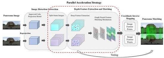
Considering the problems of the nonlinear distortion of panoramic images and the considerable time consumption of deep learning methods, the panoramic images are first mapped to virtual panoramic spheres [35] through the Equirectangular Projection Model. Then, the Improved Cube Projection Model is used to transform the panoramic sphere in different directions and reproject the panoramic image onto the perspective image with slight distortion in six directions (front, back, left, right, top, and bottom) to realize the correction of the panoramic image. The Superpoint (SP) deep feature extraction algorithm is used to extract features from all directions, and the graph neural network Superglue (SG) matching algorithm is used to search and match the extracted features. The best matching-point pairs are output, and the algorithm is accelerated by processing six split-frame images simultaneously. Finally, the matching points on the image in each direction are mapped back to the panoramic image via coordinate inverse mapping. The solution framework of the matching algorithm is shown in Figure 2.
2.2. Panoramic Projection Model
2.2.1. Equirectangular Projection
The latitude and longitude coordinates on the virtual panoramic sphere are mapped to the vertical and horizontal coordinates on the plane. After the panoramic image has been unfolded into a plane, its width is twice its height, and there is a one-to-one mapping relationship between any point p on the spherical panoramic image and the corresponding P point on the flat panoramic image, as shown in Figure 3.
Formula (1) presents the relationship between the spherical polar coordinates of point (,,R) and the flat panoramic image pixel coordinates of p (x, y). Formula (2) describes the correspondence between the spherical polar coordinate system and the spherical right-angle coordinate system [36].
where R is the radius of the sphere, W is the length of the plane image, is the angle between and plane, and is the angle between the pendant and .
Through a simple derivation based on Formulas (1) and (2), the relationship between the flat panoramic image pixel coordinates p(x, y) and the spherical panoramic image space coordinate system coordinates P(X,Y,Z) on the sphere can be obtained as follows:
2.2.2. Improved Cube Projection Model
The Traditional Cube Projection Model [37] maps the virtual panoramic sphere onto the six surfaces of the externally cut cube to generate six perspective images, as shown in Figure 4. The virtual panorama sphere is first mapped to the cube surface using the geometric relationship, and then the cube surface is converted into a perspective image through coordinate transformation. Finally, the mapping relationship between the virtual panoramic sphere and the perspective image is established.
The key to finding the virtual panoramic spherical image points corresponding to the cube image points is to determine which surface of the cube each virtual panoramic spherical image point should be mapped to. Formula (4) is the judgment formula. , , and must have values of +1 or −1, and the virtual panoramic spherical image point must be located in the cube image of one of the six sides. For example, if = +1, the virtual spherical point should be mapped to the positive Y, which is the right face of the cube [38].
where , which means the maximum absolute value of the three coordinates X, Y, and Z.
In the traditional model, the origin of the cube mapping coordinate system is the center of the image, whereas in the improved model, the upper left corner of the image is the origin. The coordinates in this coordinate system are recalculated, and the cube mapping is converted into a perspective image. The standard mapping relationship of the geometric mapping from the spherical panoramic image to the ordinary image is determined.
As shown in Figure 5, if the length and width of the plane image are W and H, respectively, Formula (5) presents the correspondence between the pixel coordinates (u,v) and the plane rectangular coordinates (x,y) [39].
Formula (6) presents the correspondence among the spherical panoramic image point coordinates (X,Y,Z), the cube image point coordinates (,,), and the coordinates of each plane pixel (u,v) (using the front example).
When = +1, the points on the virtual sphere are mapped to the front [40].
However, the Traditional Cube Projection Model has problems. It is discontinuous between split-frame images. Therefore, after two panoramic images have been reprojected, the split-frame images are matched one-by-one. Some of the split-frame images may not have high overlap rates, and the matching effect may be unsatisfactory, as shown in Figure 6.
To address this situation, the Traditional Cube Projection Model was extended to increase the overlap rate between the split-frame images after reprojection, which can result in a better matching effect when the split-frame images are matched one-by-one, as shown in Figure 7a.
As shown in Figure 7b, following the above idea, the vertical FOV remains unchanged and the horizontal FOV is increased, so that better matching results can be obtained for the split-frame images with low overlap rates and difficult matching.
2.3. Split-Frame Image Feature Extraction Algorithm
The Split-Frame Image Feature Extraction algorithm achieves the simultaneous extraction of features in six split-frame images, each extracted independently using the SP algorithm. The structure of local feature keys and descriptors is shown in Figure 8. The SP Extract Feature Network algorithm consists of three modules: the Encoder, Interest Point Decoder, and Descriptor Decoder. The Encoder is built from a lightweight fully convolutional network modified by [41], which replaces the fully connected layer at the end of the traditional network with a convolutional layer. The main function of the Encoder is to extract features after the dimensionality reduction of the image, reducing the number of subsequent mesh calculations. Through the Encoder, the input image is encoded as the intermediate tensor .
The Interest Point Decoder consists mainly of point-by-point convolutional layers, Softmax activation functions, and tensor transformation functions. In the Interest Point Decoder, the main function of the convolutional layer is to transform the intermediate tensor output of the decoder into a feature graph and then use the Softmax activation function to obtain a feature image of . Using the tensor transformation function, the subpixel convolution method is substituted for the traditional upsampling method, which has the advantage of reducing the calculation workload of the model while restoring the resolution of the feature image. The characteristic curve of can be directly flattened to the thermal map tensor of the eigencurve, and each channel vector in the eigencurve corresponds to the thermal value of the 8 × 8 region of the thermal map. Finally, each value of the heat map tensor characterizes the probability magnitude of the pixel as a feature point.
The Descriptor Decoder is used to generate semi-dense descriptor feature maps, first through the convolutional layer output , as semi-dense descriptors (that is, one output for every eight pixels). Semi-dense descriptors can significantly reduce the memory consumption and computational burden while maintaining the operational efficiency. The decoder then double-triple-interpolates the descriptor to achieve pixel-level accuracy, and finally, the dense feature map is obtained via normalization.
Because the SP algorithm uses Homographic Adaption to improve the generalization ability of the network during training, it has good adaptability to rotation, scaling, and certain distortions. It obtains good feature extraction results on six split-frame images.
2.4. Attentional Graph Neural Network Feature Matching
The six split-frame images of the two panoramic images after the SP algorithm has extracted the deep features are matched using the SG algorithm for deep features. The framework of the SG algorithm is shown in Figure 9.
The SG is a feature matching and outer point culling network, which enhances the features of key points using a GNN and transforms feature matching problems into solutions for differentially optimized transfer problems. The algorithm consists of two main modules: the Attentional Graph Neural Network and the Optimal Matching Layer. The Attentional Graph Neural Network integrates the location information of the feature points with the description subinformation after coding and then interweaves the L wheel through the attention layer and the cross attention layer, aggregating the context information within the image and between the images to obtain a more specific feature matching vector f for matching.
The Optimal Matching Layer calculates the internal product between the feature matching vectors f using Formula (7) to obtain the matching degree score matrix , where M and N represent the numbers of feature points in images A and B, respectively.
where represents the inner product, and and are the feature matching vectors of images A and B, respectively, which are output by the feature enhancement module.
Because some feature points are affected by problems such as occlusion and there is no matching point, the algorithm uses the garbage-bin mechanism, as indicated by Formula (8). The garbage bin consists of a new row and column based on the score matrix, which is used to determine whether the feature has a matching point. SuperGlue treats the final matching result as an allocation problem, constructs the optimization problem by calculating the allocation matrix and the scoring matrix S, and solves P by maximizing the overall score , , . The optimal feature assignment matrix P is quickly and iteratively solved using the Sinkhorn algorithm; thus, the optimal match is obtained.
where N and M represent the bins in A and B, respectively. The matching number of each bin is identical to the number of key points in the other group.
2.5. Coordinate Inverse Mapping Algorithm
As shown in Figure 10a, the coordinates of the corresponding P on the virtual panoramic sphere are calculated using the split-frame image coordinates (i,j).
Then, the P coordinates are used to calculate the corresponding latitude and longitude.
According to the latitude and longitude, the index coordinates of P (I,J) of the panoramic image corresponding to the latitude and longitude are found in the panorama using the Equirectangular Projection Model. Using Formula (11), the coordinates of the feature points of the perspective image can be mapped back to the panoramic image.
In the Improved Cube Projection Model, because we increase the overlap of adjacent split-frame images, split-frame images in multiple directions may match a pair of image points with the same name at the same time. Therefore, we employ a simple voting mechanism [42] in the process of mapping the binning image coordinates back to the panoramic image.
When multiple coordinates mapped back to the panoramic image are within a certain threshold, these points are considered to be the same image point, and the voting mechanism is triggered. The Euclidean distance between the midpoint of the original split image and the image center point is calculated separately. A shorter distance to the image principal point corresponds to a smaller aberration. Therefore, a shorter distance corresponds to a higher score, and the panoramic coordinate is selected as the final coordinate.
where is the center of image.
3. Results and Discussion
The details regarding the experimental data are presented in Table 1. Three types of test data were used: indoor panoramic images, outdoor panoramic images, and underground panoramic images. The resolutions were identical, but the types of images differed, giving very representative data for the test algorithm.
Figure 11 shows thumbnails of the test images. The first group was taken indoors, and the image displacement was small, but the aberration was large. The second group was shot outdoors. The image displacement was larger than that for the first group, and the aberration was slightly smaller than that for the first group. The third group was shot in an underground garage, and some areas were shadowed or poorly lit.
To validate the proposed algorithm, multiple sets of panoramic image data were used to conduct experiments, and the results were compared with those of other algorithms. The deep learning model was implemented using the PyTorch framework. The SP and SG models adopted the official pretraining weight file. The computer used for the test was a Lenovo Y9000K Notebook. The CPU was i7-10875H, and the graphics card was GeForce RTX 2080. The implementation language was Python, the operating system was Ubuntu 20.04 64-bit, and the CUDA Toolkit version was 11.3. Relevant experiments were conducted for all aspects of the proposed framework, and the experimental results were analyzed using different evaluation metrics.
3.1. Distortion Correction Effect
The reprojection of the panoramic image into the split-frame images in six directions is a process similar to perspective transformation. Figure 12 shows the transformation of the image after reprojection. From the experimental results, it can be seen that the reprojected image satisfies the basic characteristics of the perspective image. The nonlinear distortion of the key buildings is basically eliminated, and the shapes of the key buildings and objects conform to their spatial geometric characteristics, which is convenient for subsequent feature extraction and matching.
3.2. Extension-Angle Test
The Traditional Cube Projection Model was used to perform an experimental verification of the proposed algorithm, and the results are shown in Figure 13a.
As shown in Figure 13a, the split-frame images in all directions are discontinuous, which led to difficulty in extracting the building features at the junction. Therefore, we adopted the strategy of model extension to enhance the continuity between the directions. Experimental validation was performed for different extension angles.
As shown in Figure 13b, the buildings that were not successfully matched before were well matched with the Improved Cube Projection Model, resulting in a more uniform and dense distribution of matching points.
We used the number of correct matching points obtained and the matching time as the main evaluation indexes. We selected extension angles of 5°, 10°, and 15° and then conducted a comparison test. The experimental results are presented in Table 2, and the experimental effect graph is shown in Figure 14. A comprehensive analysis indicated that the 10° extension angle achieved better results for image matching than the 5° extension angle at the expense of a lower time efficiency. The 15° extension angle increased the number of matching points slightly compared with the 10° extension angle, but the time efficiency decreased significantly. Therefore, in subsequent experiments, the 10° extension angle was adopted.
3.3. Voting Mechanism Effect
The matching experiments were first performed directly using the Traditional Cube Projection Model after applying the extension angle, and the problem of duplicate matching points appeared in four regions, as shown in Figure 15. The details are shown in Figure 16a. There are many duplicate matching points.
As shown in Figure 16b, the voting mechanism designed in this study solves this problem perfectly. The feature points of the remapped panoramic image are accurate, and no duplicate matching points are generated.
3.4. Adaptability of the Algorithm
As shown in Figure 17, several other algorithms do not extract features or extract fewer feature points in the region with large indoor distortion. The proposed algorithm extracted uniform and dense feature points in the area with large indoor distortion and performed well.
The red box in Figure 18 shows an environment with poor lighting conditions, and the other algorithms in the test experiments were unable to extract features in this area. In contrast, the proposed algorithm performed well because of the SP and SG deep learning approach with a strong generalization ability and good adaptability to different environments.
3.5. Feature Matching Number and Precision
The correct matching point was determined as shown in the formula:
where is the true location of the feature point. is the actual position of the feature point calculated by the algorithm.
The proposed method was compared with the SIFT, ASIFT, and Improved ASIFT [43] algorithms using three sets of experimental data, and the experimental results are shown in Table 3. The experimental results of various algorithms for image feature extraction and matching are shown in Figure 19.
Table 3 shows that SIFT matching takes the longest amount of time, eight times longer than the ASIFT algorithm and thirty times longer than the improved ASIFT algorithm and the algorithm in this paper. The algorithm in this paper has the highest accuracy with the shortest matching elapsed time. It is 5% higher than the improved ASIFT, 20% higher than the ASIFT algorithm, and 55% higher than the SIFT algorithm.
Figure 19 and Figure 20 shows that the SIFT algorithm obtained a small number of matching points with an uneven distribution. The ASIFT algorithm obtained the largest number of matching points, but the distribution was not uniform, and the distortion area could not extract enough feature points. The Improved ASIFT algorithm had a more uniform distribution of matching points but a smaller number. Our algorithm extracted more matching points than the Improved ASIFT with a more uniform and reasonable distribution.
4. Conclusions and Discussion
Panoramic image matching is a challenging task. Faced with the interference caused by the large nonlinear distortion of panoramic images, it is difficult to achieve results comparable to those for perspective images using traditional feature extraction and matching algorithms. Therefore, we used the Improved Cube Projection Model for aberration correction to improve the matching effect of panoramic images. The image matching time was reduced via the acceleration strategy of processing split-frame images simultaneously.
We extended the Traditional Cube Projection Model to address the shortcomings of discontinuity among the split-frame images of the Traditional Cube Projection Model. More uniform and robust matching was achieved on the basis of sacrificing time efficiency. Using the SP and SG deep learning approach, the powerful generalization ability of the deep learning network was utilized to maintain good results in cases of large distortions or poor lighting conditions.
We confirmed the feasibility of using CNNs for panoramic image matching and made targeted improvements to address shortcomings in the application process, which yielded good matching results. This study provides new ideas and methods for large-scale 3D scene reconstruction using panoramic images. In this paper, the CNN was used to achieve a good matching effect and was shown to accurately describe the relative position relationship between images and has important potential value in several fields. It provides an accurate viewpoint and position relationship for building digital cities and facilitates the construction of more complete and detailed digital city models. At the same time, it can acquire a large number of image points with the same name in the image, which provides a large number of virtual control points for SLAM and improves its accuracy when building maps.
Although the proposed method in this paper achieved a good performance level, there are still several limitations in our method. Because the proposed algorithm reprojects the panoramic image onto split-frame images in different directions, the corresponding directional split-frame images are matched one-by-one. Therefore, it is not suitable for images with different imaging modes. When composing a panoramic image, one imaging mode is that the image captured by the forward-facing lens is in the center of the panoramic image; the other imaging mode is that the image captured by the forward-facing lens is at the edge of the panoramic image. When the proposed algorithm was tested on such images, the results were unsatisfactory.
The idea of converting panoramic images to perspective images is still used to implement CNNs for panoramic images. In future research, we will explore the idea of using panoramic image datasets directly to train CNN networks to achieve a better matching performance. We will also continue to study other work after matching, so as to play a more important role in digital city or 3D reconstruction.
Author Contributions
T.G., C.L. and L.W. conceived the approach and designed the experiments; W.H. performed the experiments and analyzed the data; F.Y. contributed to the data analysis; T.G. wrote the paper; and Z.W. reviewed the paper. All authors have read and agreed to the published version of the manuscript.
Funding
This research received no external funding.
Data Availability Statement
Data will be available upon request to the first author.
Conflicts of Interest
The authors declare no conflict of interest.
References
- Bakirman, T.; Gumusay, M.U. Integration of Custom Street View and Low Cost Motion Sensors. Int. J. Eng. Geosci. 2020, 5, 66–72. [Google Scholar] [CrossRef]
- Peng, C.; Chen, B.Y.; Tsai, C.H. Integrated google maps and smooth street view videos for route planning. In Proceedings of the 2010 International Computer Symposium (ICS2010), Tainan, Taiwan, 16–18 December 2010; IEEE: Piscataway, NJ, USA, 2010; pp. 319–324. [Google Scholar]
- Bertel, T.; Campbell, N.D.; Richardt, C. Megaparallax: Casual 360 panoramas with motion parallax. IEEE Trans. Vis. Comput. Graph. 2019, 25, 1828–1835. [Google Scholar] [CrossRef] [PubMed]
- Golodetz, S.; Cavallari, T.; Lord, N.A.; Prisacariu, V.A.; Murray, D.W.; Torr, P.H. Collaborative large-scale dense 3d reconstruction with online inter-agent pose optimisation. IEEE Trans. Vis. Comput. Graph. 2018, 24, 2895–2905. [Google Scholar] [CrossRef] [Green Version]
- Yang, S.; Li, B.; Liu, M.; Lai, Y.K.; Kobbelt, L.; Hu, S.M. Heterofusion: Dense scene reconstruction integrating multi-sensors. IEEE Trans. Vis. Comput. Graph. 2019, 26, 3217–3230. [Google Scholar] [CrossRef] [PubMed] [Green Version]
- Zhang, H.; Xu, F. Mixedfusion: Real-time reconstruction of an indoor scene with dynamic objects. IEEE Trans. Vis. Comput. Graph. 2017, 24, 3137–3146. [Google Scholar] [CrossRef] [PubMed]
- Cha, Y.W.; Price, T.; Wei, Z.; Lu, X.; Rewkowski, N.; Chabra, R.; Qin, Z.; Kim, H.; Su, Z.; Liu, Y.; et al. Towards fully mobile 3D face, body, and environment capture using only head-worn cameras. IEEE Trans. Vis. Comput. Graph. 2018, 24, 2993–3004. [Google Scholar] [CrossRef]
- Yang, X.; Zhou, L.; Jiang, H.; Tang, Z.; Wang, Y.; Bao, H.; Zhang, G. Mobile3DRecon: Real-time monocular 3D reconstruction on a mobile phone. IEEE Trans. Vis. Comput. Graph. 2020, 26, 3446–3456. [Google Scholar] [CrossRef]
- Xu, L.; Cheng, W.; Guo, K.; Han, L.; Liu, Y.; Fang, L. Flyfusion: Realtime dynamic scene reconstruction using a flying depth camera. IEEE Trans. Vis. Comput. Graph. 2019, 27, 68–82. [Google Scholar] [CrossRef]
- Sitzmann, V.; Serrano, A.; Pavel, A.; Agrawala, M.; Gutierrez, D.; Masia, B.; Wetzstein, G. Saliency in VR: How do people explore virtual environments? IEEE Trans. Vis. Comput. Graph. 2018, 24, 1633–1642. [Google Scholar] [CrossRef] [Green Version]
- Stotko, P.; Krumpen, S.; Hullin, M.B.; Weinmann, M.; Klein, R. SLAMCast: Large-scale, real-time 3D reconstruction and streaming for immersive multi-client live telepresence. IEEE Trans. Vis. Comput. Graph. 2019, 25, 2102–2112. [Google Scholar] [CrossRef] [Green Version]
- Zhang, J.; Gui, M.; Wang, Q.; Liu, R.; Xu, J.; Chen, S. Hierarchical topic model based object association for semantic SLAM. IEEE Trans. Vis. Comput. Graph. 2019, 25, 3052–3062. [Google Scholar] [CrossRef] [PubMed]
- Eitz, M.; Hildebrand, K.; Boubekeur, T.; Alexa, M. Sketch-based image retrieval: Benchmark and bag-of-features descriptors. IEEE Trans. Vis. Comput. Graph. 2010, 17, 1624–1636. [Google Scholar] [CrossRef] [PubMed] [Green Version]
- Cheng, Z.Q.; Chen, Y.; Martin, R.R.; Lai, Y.K.; Wang, A. Supermatching: Feature matching using supersymmetric geometric constraints. IEEE Trans. Vis. Comput. Graph. 2013, 19, 1885–1894. [Google Scholar] [CrossRef] [PubMed] [Green Version]
- Heiberg, E.; Ebbers, T.; Wigstrom, L.; Karlsson, M. Three-dimensional flow characterization using vector pattern matching. IEEE Trans. Vis. Comput. Graph. 2003, 9, 313–319. [Google Scholar] [CrossRef]
- Andersen, D.; Villano, P.; Popescu, V. AR HMD guidance for controlled hand-held 3D acquisition. IEEE Trans. Vis. Comput. Graph. 2019, 25, 3073–3082. [Google Scholar] [CrossRef]
- Tsai, V.J.; Chang, C.T. Three-dimensional positioning from Google street view panoramas. Iet Image Process. 2013, 7, 229–239. [Google Scholar] [CrossRef] [Green Version]
- Lowe David, G. Distinctive image features from scale-invariant interest points. Int. J. Comput. Vis. 2004, 60, 91–100. [Google Scholar] [CrossRef]
- Bay, H.; Ess, A.; Tuytelaars, T.; Van Gool, L. Speeded-Up Robust Features (SURF). Comput. Vis. Image Underst. 2008, 110, 346–359, Similarity Matching in Computer Vision and Multimedia. [Google Scholar] [CrossRef]
- Rublee, E.; Rabaud, V.; Konolige, K.; Bradski, G. ORB: An efficient alternative to SIFT or SURF. In Proceedings of the 2011 International Conference on Computer Vision, Barcelona, Spain, 6–13 November 2011; pp. 2564–2571. [Google Scholar] [CrossRef]
- Calonder, M.; Lepetit, V.; Strecha, C.; Fua, P. BRIEF: Binary Robust Independent Elementary Features. In Proceedings of the Computer Vision–ECCV 2010, Heraklion, Greece, 5–11 September 2010; Daniilidis, K., Maragos, P., Paragios, N., Eds.; Springer: Berlin/Heidelberg, Germany, 2010; pp. 778–792. [Google Scholar]
- Wu, J.; Cui, Z.; Sheng, V.S.; Zhao, P.; Su, D.; Gong, S. A Comparative Study of SIFT and its Variants. Meas. Sci. Rev. 2013, 13, 122–131. [Google Scholar] [CrossRef] [Green Version]
- Muja, M.; Lowe, D.G. Scalable nearest neighbor algorithms for high dimensional data. IEEE Trans. Pattern Anal. Mach. Intell. 2014, 36, 2227–2240. [Google Scholar] [CrossRef]
- Chen, J.; Li, Q.; Peng, Q.; Wong, K.H. CSIFT based locality-constrained linear coding for image classification. Pattern Anal. Appl. 2015, 18, 441–450. [Google Scholar] [CrossRef] [Green Version]
- Haehn, D.; Tompkin, J.; Pfister, H. Evaluating ‘graphical perception’with CNNs. IEEE Trans. Vis. Comput. Graph. 2018, 25, 641–650. [Google Scholar] [CrossRef] [PubMed] [Green Version]
- Li, G.; Wang, J.; Shen, H.W.; Chen, K.; Shan, G.; Lu, Z. Cnnpruner: Pruning convolutional neural networks with visual analytics. IEEE Trans. Vis. Comput. Graph. 2020, 27, 1364–1373. [Google Scholar] [CrossRef] [PubMed]
- Zagoruyko, S.; Komodakis, N. Learning to compare image patches via convolutional neural networks. In Proceedings of the IEEE Conference on Computer Vision and Pattern Recognition, Boston, MA, USA, 7–12 June 2015; pp. 4353–4361. [Google Scholar]
- Ye, F.; Su, Y.; Xiao, H.; Zhao, X.; Min, W. Remote sensing image registration using convolutional neural network features. IEEE Geosci. Remote Sens. Lett. 2018, 15, 232–236. [Google Scholar] [CrossRef]
- Yi, K.M.; Trulls, E.; Lepetit, V.; Fua, P. Lift: Learned invariant feature transform. In Proceedings of the European Conference on Computer Vision, Amsterdam, The Netherlands, 11–14 October 2016; Springer: Berlin/Heidelberg, Germany, 2016; pp. 467–483. [Google Scholar]
- DeTone, D.; Malisiewicz, T.; Rabinovich, A. Superpoint: Self-supervised interest point detection and description. In Proceedings of the IEEE Conference on Computer Vision and Pattern Recognition Workshops, Salt Lake City, UT, USA, 18–22 June 2018; pp. 224–236. [Google Scholar]
- Noh, H.; Araujo, A.; Sim, J.; Weyand, T.; Han, B. Large-scale image retrieval with attentive deep local features. In Proceedings of the IEEE International Conference on Computer Vision, Venice, Italy, 22–29 October 2017; pp. 3456–3465. [Google Scholar]
- Dusmanu, M.; Rocco, I.; Pajdla, T.; Pollefeys, M.; Sivic, J.; Torii, A.; Sattler, T. D2-net: A trainable cnn for joint detection and description of local features. arXiv 2019, arXiv:1905.03561. [Google Scholar]
- Sarlin, P.E.; DeTone, D.; Malisiewicz, T.; Rabinovich, A. Superglue: Learning feature matching with graph neural networks. In Proceedings of the IEEE/CVF Conference on Computer Vision and Pattern Recognition, Seattle, WA, USA, 13–19 June 2020; pp. 4938–4947. [Google Scholar]
- Yang, W.; Qian, Y.; Kämäräinen, J.K.; Cricri, F.; Fan, L. Object detection in equirectangular panorama. In Proceedings of the 2018 24th International Conference on Pattern Recognition (ICPR), Beijing, China, 20–24 August 2018; IEEE: Piscataway, NJ, USA, 2018; pp. 2190–2195. [Google Scholar]
- Liu, S.; Chen, J.; Sun, M.; Zhao, L.; Wei, X. A fast epipolar line matching method based on 3D spherical panorama. IEEE Access 2019, 8, 11754–11760. [Google Scholar] [CrossRef]
- Startsev, M.; Dorr, M. 360-aware saliency estimation with conventional image saliency predictors. Signal Process. Image Commun. 2018, 69, 43–52. [Google Scholar] [CrossRef]
- Li, J.; Wen, Z.; Li, S.; Zhao, Y.; Guo, B.; Wen, J. Novel tile segmentation scheme for omnidirectional video. In Proceedings of the 2016 IEEE International Conference on Image Processing (ICIP), Phoenix, AZ, USA, 25–28 September 2016; IEEE: Piscataway, NJ, USA, 2016; pp. 370–374. [Google Scholar]
- Zhixuan, W.; Ruofei, Z.; Donghai, X. Automatically measuring the coordinates of streetlights in vehicle-borne spherical images. J. Image Graph. 2018, 23, 1371–1381. [Google Scholar]
- Wang, F.E.; Yeh, Y.H.; Sun, M.; Chiu, W.C.; Tsai, Y.H. Bifuse: Monocular 360 depth estimation via bi-projection fusion. In Proceedings of the IEEE/CVF Conference on Computer Vision and Pattern Recognition, Seattle, WA, USA, 13 June 2020; pp. 462–471. [Google Scholar]
- Wang, Y.; Cai, S.; Li, S.J.; Liu, Y.; Guo, Y.; Li, T.; Cheng, M.M. Cubemapslam: A piecewise-pinhole monocular fisheye slam system. In Proceedings of the Asian Conference on Computer Vision, Perth, Australia, 2–6 December 2018; Springer: Berlin/Heidelberg, Germany, 2018; pp. 34–49. [Google Scholar]
- Simonyan, K.; Zisserman, A. Very deep convolutional networks for large-scale image recognition. arXiv 2014, arXiv:1409.1556. [Google Scholar]
- Imik Tanyildizi, N.; Tanyildizi, H. Estimation of voting behavior in election using support vector machine, extreme learning machine and deep learning. Neural Comput. Appl. 2022, 34, 17329–17342. [Google Scholar] [CrossRef]
- Fu, H.; Xie, D.; Zhong, R.; Wu, Y.; Wu, Q. An improved ASIFT algorithm for indoor panorama image matching. In Proceedings of the Ninth International Conference on Digital Image Processing (ICDIP 2017), Hong Kong, China, 19–22 May 2017; SPIE: Bellingham, WA, USA, 2017; Volume 10420, pp. 285–292. [Google Scholar]
Figure 1.
The panoramic camera combines the lens distribution method and the stitching order of the shooting images as well as the panoramic image generated by the stitching (take the panoramic camera of the Google Panorama car as an example, different numbers in the picture are different camera lens numbers).

Figure 2.
Overview of the proposed matching method, which consists of three main parts. The first part involves correcting the aberrations of the split-direction image and mapping the panoramic image into six split-frame perspective images with small aberrations via the Improved Cube Projection Model. The second part involves the feature extraction and matching of the split-frame images using the deep feature extraction and matching algorithm. The third part involves coordinate inverse mapping, where the coordinates of the matching points of the split-frame image are mapped back to the panoramic image. The ambiguity problem in the mapping process is solved by the voting mechanism. The algorithm is accelerated by processing the split-frame images in parallel.

Figure 3.
Mapping of the relationship between the spherical panoramic image and flat panoramic image. Point p on the spherical panoramic image and point P on the flat panoramic image are unique mapping correspondence points.
Figure 3.
Mapping of the relationship between the spherical panoramic image and flat panoramic image. Point p on the spherical panoramic image and point P on the flat panoramic image are unique mapping correspondence points.

Figure 4.
Correspondence between the image segments of the panoramic sphere and the Cube Projection Model and the coordinate systems of the generated split-frame images.
Figure 4.
Correspondence between the image segments of the panoramic sphere and the Cube Projection Model and the coordinate systems of the generated split-frame images.

Figure 5.
Correspondence between the image segments of the panoramic sphere and the Cube Projection Model and the coordinate systems of the generated split-frame images.
Figure 5.
Correspondence between the image segments of the panoramic sphere and the Cube Projection Model and the coordinate systems of the generated split-frame images.

Figure 6.
Four split-frame images generated by the Traditional Cube Projection Model. The images marked in red have low overlap rates.
Figure 6.
Four split-frame images generated by the Traditional Cube Projection Model. The images marked in red have low overlap rates.

Figure 7.
(a) Side view: the overlap is the increased overlap between cameras 1 and 2. (b) Top view: the FOV of Camera 1 is extended by from 90°.
Figure 7.
(a) Side view: the overlap is the increased overlap between cameras 1 and 2. (b) Top view: the FOV of Camera 1 is extended by from 90°.

Figure 8.
SP feature extraction model, which mainly consists of the Encoder, Interest Point Decoder, and Descriptor Decoder [30].
Figure 8.
SP feature extraction model, which mainly consists of the Encoder, Interest Point Decoder, and Descriptor Decoder [30].

Figure 9.
SG algorithm framework. There are two main parts: the Attentional Graph Neural Network, which is used to enhance the matching-point features, and the Optimal Matching Layer, where the optimal matching result is selected [33].
Figure 9.
SG algorithm framework. There are two main parts: the Attentional Graph Neural Network, which is used to enhance the matching-point features, and the Optimal Matching Layer, where the optimal matching result is selected [33].

Figure 10.
Coordinate mapping schematic. On the left (a) is P on the split-frame image. On the right (b) is the corresponding P′ on the panoramic image.
Figure 10.
Coordinate mapping schematic. On the left (a) is P on the split-frame image. On the right (b) is the corresponding P′ on the panoramic image.

Figure 11.
Thumbnails of the test image.

Figure 12.
Comparison of the images before and after correction. The red boxed area is the area to be corrected, and the right side is the corrected effect of the area.
Figure 12.
Comparison of the images before and after correction. The red boxed area is the area to be corrected, and the right side is the corrected effect of the area.

Figure 13.
Experimental (a) renderings before the model improvement. (b) renderings after the model improvement. The red box shows the key contrast areas for the matching effect.
Figure 13.
Experimental (a) renderings before the model improvement. (b) renderings after the model improvement. The red box shows the key contrast areas for the matching effect.

Figure 14.
Experimental results for different extension angles. The red boxed area is the junction of the Conventional Cube Model split image. As shown, the 10° extension angle was better than the 5° extension angle, and the 15° extension angle was hardly better than the 10° extension angle.
Figure 14.
Experimental results for different extension angles. The red boxed area is the junction of the Conventional Cube Model split image. As shown, the 10° extension angle was better than the 5° extension angle, and the 15° extension angle was hardly better than the 10° extension angle.

Figure 15.
(a) The effect before voting at the indoor. (b) The effect before voting at the outdoor. The red box is selected as the problem area with duplicate mappings in the inverse coordinate mapping.
Figure 15.
(a) The effect before voting at the indoor. (b) The effect before voting at the outdoor. The red box is selected as the problem area with duplicate mappings in the inverse coordinate mapping.

Figure 16.
The effect of voting. (a) The feature points marked in blue are repeatedly mapped in the coordinate inverse mapping. (b) Optimal solution obtained by the voting algorithm.
Figure 16.
The effect of voting. (a) The feature points marked in blue are repeatedly mapped in the coordinate inverse mapping. (b) Optimal solution obtained by the voting algorithm.

Figure 17.
Match results for areas with larger distortions.

Figure 18.
Experimental results of our algorithm under dark light conditions.

Figure 19.
Image feature extraction and matching experimental renderings with various algorithms.

Figure 20.
Visualization of time and accuracy parameters.


Table 1.
Summary of testing datasets.
| Group ID | 1 | 2 | 3 |
|---|---|---|---|
| Image type | indoor | outdoor | underground |
| Image size | 5376 × 2688 | 5376 × 2688 | 5376 × 2688 |
| Features | Close distance, | large distortion | Large interimage |
| displacement | Large differences | in lighting conditions |
Table 2.
Results of the angle extension experiment.
| Group | Indoor | Outdoor | Underground | |||
|---|---|---|---|---|---|---|
| Degree | Number | Time (s) | Number | Time (s) | Number | Time (s) |
| 5° | 1369 | 6.4 | 1675 | 8.2 | 882 | 5.9 |
| 10° | 1420 | 7.1 | 1891 | 8.9 | 1015 | 6.4 |
| 15° | 1386 | 11.7 | 1915 | 15.9 | 1035 | 9.6 |
Table 3.
Comparison of the results of the matching methods.
| Group | Methods | Pairs | Correct Pairs | Time (s) | Accuracy (%) |
|---|---|---|---|---|---|
| Indoor | SIFT | 5201 | 634 | 307 | 12.2 |
| ASIFT | 8195 | 3188 | 31.7 | 38.9 | |
| Improved ASIFT | 1775 | 1157 | 8.2 | 65.2 | |
| Ours | 1420 | 994 | 7.1 | 70.0 | |
| Outdoor | SIFT | 4588 | 371 | 196.5 | 8.1 |
| ASIFT | 6093 | 4445 | 31.8 | 73.0 | |
| Improved ASIFT | 1323 | 940 | 9.5 | 71.1 | |
| Ours | 1891 | 1433 | 8.9 | 75.8 | |
| Under. | SIFT | 3654 | 470 | 136.5 | 12.9 |
| ASIFT | 4987 | 2153 | 16.6 | 43.2 | |
| Improved ASIFT | 647 | 500 | 7.1 | 77.3 | |
| Ours | 1015 | 793 | 6.4 | 78.1 |
Disclaimer/Publisher’s Note: The statements, opinions and data contained in all publications are solely those of the individual author(s) and contributor(s) and not of MDPI and/or the editor(s). MDPI and/or the editor(s) disclaim responsibility for any injury to people or property resulting from any ideas, methods, instructions or products referred to in the content. |
© 2023 by the authors. Licensee MDPI, Basel, Switzerland. This article is an open access article distributed under the terms and conditions of the Creative Commons Attribution (CC BY) license (https://creativecommons.org/licenses/by/4.0/).
Share and Cite
MDPI and ACS Style
Gao, T.; Lan, C.; Wang, L.; Huang, W.; Yao, F.; Wei, Z. Leveraging CNNs for Panoramic Image Matching Based on Improved Cube Projection Model. Remote Sens. 2023, 15, 3411. https://0-doi-org.brum.beds.ac.uk/10.3390/rs15133411
AMA Style
Gao T, Lan C, Wang L, Huang W, Yao F, Wei Z. Leveraging CNNs for Panoramic Image Matching Based on Improved Cube Projection Model. Remote Sensing. 2023; 15(13):3411. https://0-doi-org.brum.beds.ac.uk/10.3390/rs15133411
Chicago/Turabian StyleGao, Tian, Chaozhen Lan, Longhao Wang, Wenjun Huang, Fushan Yao, and Zijun Wei. 2023. "Leveraging CNNs for Panoramic Image Matching Based on Improved Cube Projection Model" Remote Sensing 15, no. 13: 3411. https://0-doi-org.brum.beds.ac.uk/10.3390/rs15133411
Note that from the first issue of 2016, this journal uses article numbers instead of page numbers. See further details here.