Mitigating the Impact of Harmful Algal Blooms on Aquaculture Using Technological Interventions: Case Study on a South African Farm

Abstract

Seafood, especially from the ocean, is now seen as a greener and more sustainable source of protein, causing an increase in its demand. This has also led to people making choices towards seafood as a replacement for carbon-intensive protein sources. As a result, the demand for seafood is growing, and as the aquaculture industry looks to increase production, keeping products safe and sustainable is imperative. There are many challenges faced by the aquaculture industry in meeting these increased demands. One such challenge is the presence of harmful algal blooms (HABs) in the ocean, which can have a major impact on aquatic life. In this paper, we look at the impact of this challenge on aquaculture and monitoring strategies whilst illustrating the potential for technological interventions to help mitigate the impact of an HAB. We will focus on Abagold Limited, a land-based marine aquaculture business that specialises in the large-scale production of abalone (Haliotis midae) based in Hermanus, South Africa. HABs are considered a threat to commercial-scale abalone farming along the South African coastline and require continuous monitoring. The most recent HAB was in February–April 2019, when the area experienced a severe red-tide event with blooms of predominantly Lingulodinium polyedrum. We present some of the monitoring strategies employing digital technologies to future-proof the industry. This article presents the development of a novel hybrid water quality forecasting model based on a TriLux multi-parameter sensor to monitor key water quality parameters. The actual experimental real water quality data from Abagold Limited show a good correlation as a basis for a forecasting model which would be a useful tool for the management of HABs in the aquaculture industry.

1. Introduction

Phytoplankton, also known as microalgae, are like terrestrial plants in that they contain chlorophyll and require sunlight to live and grow. Most phytoplankton are buoyant and float in the upper part of the ocean, where sunlight penetrates the water. Marine algal blooms are commonly referred to as red tides or harmful algal blooms (HABs), but they occur in a variety of colours depending on the type(s) of algae present. Only a small number of species have the capacity to form harmful blooms, but when they do, the effects can be severe for coastal resources, local economies, and public health. Harmful algal blooms (HABs) occur when algae grow out of control and sometimes produce toxins harmful to aquatic life and, in some cases, to humans. Hallegraeph [1] categorises them into three broad groups. Group one is harmless (i.e., non-toxin-producing), colourless algae that can also form a bloom and deplete a waterbody of oxygen, killing aquatic life; an example is the dinoflagellates taxon, specifically, Akashiwo sanguinea. The second group includes species which produce potent toxins that can affect humans, causing a variety of gastrointestinal and neurological illnesses; the most common example includes paralytic shellfish poisoning (PSP) caused by dinoflagellates Alexandrium catenella [2]. However, the focus here is on the third category of HABs, which produce toxins harmful to aquatic life. While wild aquatic animals have the option of moving away when such a bloom occurs, farmed aquatic life is more vulnerable to such HABs.

These types of algae are complex, and their ability to devastate aquaculture farms has posed a significant challenge to the industry’s sustainability. There are several mechanisms through which HABs threaten the viability of cultured organisms, primarily through the dysfunction of the respiratory system by mechanically damaging the gill epithelium or the induction of hypoxic or anoxic conditions during bloom degradation. These conditions fuel microbial respiration, resulting in oxygen depletion. Additionally, toxins produced by specific algal species compromise the sensor motor function in adult and larval fish, impeding essential behaviours such as feeding [3]. Furthermore, these toxins disrupt osmoregulatory processes, leading to an increase in blood variables of sodium (Na⁺), potassium (K⁺), and chloride (Cl⁻), resulting in mortality [4]. Moreover, the accumulation of these toxins within cultured organisms poses a significant public health risk, particularly shellfish poisoning, should toxin concentrations exceed regulatory limits [5]. Therefore, aquaculture systems rely on early warning systems to manage blooms effectively, minimising the risk of rapid fish loss and preserving public health, as successful management requires a complex process involving various monitoring and control techniques. The frequency and intensity of these blooms have developed into a global concern over the past few years. The impact of blooms is not often quantified except in cases where it has resulted in massive mortalities of cultured animals and significant economic losses. The more notable globally iconic blooming events and their impact on the aquaculture industry are summarised in

Table 1. Harmful algal bloom events attributed to known species of harmful algae and their impact on aquaculture.

HAB	Toxin	Cultured Animal	Location	Impact	Year	Reference
Chrysochromulina leadbeateri	Not Toxic/No Data	Salmon	Northern Norway	It was estimated to have killed 8 million salmon, a total of 14,000 tonnes with a value of over EUR 80 million. Fish death was sudden with gill damage frequently observed.	2019	John, U. et al., 2022 [6]
Karenia mikimotoi	Ichthyotoxins	Mussel	St Austell Bay and Lyme Bay, English Channel, UK	This led to an 18-week harvesting ban, costing over GBP 1 million in loss of sales. The okadaic acid accumulation in the shellfish exceeded regulatory limits.	2018	Ross Brown et al., 2022 [7]
Noctiluca scintillans	Non- toxic
Dinophysis acuminata	Pectenotoxins Okadaic acid
Dinophysis acuta
Heterosigma akashiwo	Not toxic/No Data	Salmon	Canada	Resulted in the deaths of more than 250,000 salmon.	2018	Robinson Matt, 2018 [8]
Gonyaulax spinifera	Yessotoxins Yessotoxins	Abalone	South Africa	Severe disruption of the gill epithelium was characterised by degeneration and necrosis. The total loss was estimated to have exceeded 250 tonnes.	2017	Pitcher et al., 2019 [9]
Lingulodinium polyedrum
Pseudochattonella verruculosa	Ichthyotoxins	Salmon	Chile	This resulted in the mortality of 39 million salmon and an economic loss of USD 800 million. Examination showed that gills were the most affected organ with significant tissue damage.	2016	Díaz et al., 2019 [5]
Alexandrium catenella	Saxitoxins	Mussel	Chile	Toxins led to harvesting closures of multiple farms in the affected areas.	2016	Anderson Donald and Rensel Jack, 2016 [10]
Alexandrium fundyense	Saxitoxin	Mussel	Scotland	These toxins result in a yearly average reduction of nearly 15% in production. This is equivalent to a loss of 1080 tonnes of shellfish per year and an economic loss of GBP 1.3 million.	2005–2015	Martino, Gianella and Davidson, 2020 [11]
Dinophysis sp.	Okadaic acid
Pseudo-nitzschia sp.	Domoic acid
Alexandrium tamarense	Saxitoxins	Mussel	Australia	Toxins led to harvesting closures of multiple fishery resources in the affected areas. The marine farming sector losses based on reductions in landed catch equated to an estimated AUD 6,308,700.	2012	Campbell et al., 2013 [12]
Prorocentrum donghaiense	Non-toxic	Scallop, Abalone	China	Caused significant loss in the mariculture industries of Zhejiang and Fujian provinces, especially in cultivated abalone. The direct economic loss was more than USD 330 million. The blooms caused cessation of feeding and stagnant growth of scallops.	2010–2012	Trainer, V.L. and Yoshida, T. (Eds.) 2014 [13]
Karenia mikimotoi	Ichthyotoxins
Cochlodinium geminatum	Ichthyotoxins
Noctiluca scintillans	Non-toxic	Mussel	China	Although this bloom is non-toxic, it accumulates and releases toxic levels of ammonia into the surrounding waters. It caused high mortalities and led to USD 32.6 thousand in economic losses.	2008	Trainer, V.L. and Yoshida, T. (Eds.) 2014 [13]
Karenia brevis	Brevotoxins	Mussel	Spain	This led to harvesting bans that reduced production.	2003–2008	Rodríguez, Villasante and Carme García-Negro, 2011 [14]
Protoceratium reticulatum	Yessotoxins	Mussel	South Africa	This led to a five-month closure of mussel harvesting.	2005	Pitcher and Louw, 2021 [15]
Alexandrium catenella	Saxitoxins	Abalone	South Africa	The toxin affected the spawning capability of the abalone and larval survival. Mortalities were recorded in the broodstock.	1999	Pitcher et al., 2001 [16]
Chaetoceros wighami	Not Toxic/No Data	Salmon	Scotland	Gills showed severe necrosis with focal hyperplasia and oedematous separation of epithelia. The economic cost was a loss of 170 tonnes of production worth GBP 408,000.	1998	Treasurer, Hannah and Cox, 2003 [17]

AUD: Australian Dollar, EUR: European Union Currency, GBP: British Pound Sterling, USD: United States Dollar.

below.

2. Harmful Algal Bloom Mitigation Technologies

Harmful algal blooms have been a major cause of concern in aquaculture and their occurrence depends on several factors including temperature, precipitation, wind, surface water conditions, the presence of nutrients (eutrophication), etc. The changing climate impacts these parameters, for example, surface water acidification stemming from increased CO₂ emissions which directly alters the surface water conditions, and perhaps more importantly their extremes [18]. However, the location and intensification, due to increasing ocean temperatures [19,20], and the composition and spread of HABs will change, making their occurrence even more unpredictable [21]. This unpredictability of HABs is a cause of concern for the aquaculture business and there is an immediate need to develop suitable digital techniques that would allow the farms to mitigate their impact.

There are various tools which have been developed to monitor, quantify, or identify HABs. This section focuses on various digital technologies that have been developed in the last few years that support the monitoring/forecasting of HABs.

2.1. Tools and Instruments

The ability to detect HABs without resorting to laboratory-based sample testing is enabled by a range of sensor technologies detecting increasing turbidity and changes in chlorophyll-related spectral responses that result from increasing phytoplankton. The implementation of a specific technology can be dependent on the spatial and temporal requirements for a specific application. For example, satellite-based remote sensors can provide measurements over large areas of the globe and show the development and distribution of HABs at regular intervals, typically measured in days. Commercial aquaculture, by contrast, requires access to real-time data to detect the onset of HABs in farming tanks and employ in situ multi-parameter sensors. A brief overview of some of the sensor options available currently is presented below.

Satellite remote sensing of HABs employs spectral measurement technologies such as the MODIS (moderate-resolution imaging spectroradiometer) and the Sentinel-2A/B optical multispectral imaging satellite. Spatial resolution is typically of the order of 10s of metres. An example of this approach is presented by Bondur et al., where satellite data are integrated with ocean temperature data to identify the causes of HABs in the coastal waters east of Kamchatka, influenced by mineral and biogenic suspensions in river runoff from the Nalycheva River [22]. A further example is provided by Bu et al., where MODIS data are integrated with meteorological factors and latitude and longitude information to create a general regression dataset for harmful algal bloom detection. The analysis by Bu et al. included data from 192 HAB events from around the world over a 20-year period [23]. One of the challenges of satellite remote sensing is variability and measurement restrictions caused by cloud cover and aerosol conditions. A satellite measurement system that aims to address these issues is the TROPOspheric Monitoring Instrument (TROPOMI), which can observe red solar-induced fluorescence (SIF) resulting from HABs. This instrument is mounted on the Copernicus Sentinel-5 Precursor satellite and offers a 5.5 km spatial resolution and near-daily global coverage [24]. Luis et al. recently presented a comparison of HAB assessments from the TROPOMI and MODIS satellites and concluded that during severe HAB conditions, red SIF was consistent with existing monitoring tools and has the potential to provide nearly double the amount of spatiotemporal fluorescence HAB information [24]. Even within satellite-based remote sensing, for a given application, there are decisions to make relating to measurement robustness, atmospheric conditions, spatial resolution, and image update rate.

Jordan et al. present an above-water reflectance system capable of monitoring aquatic ecosystems with the addition of a hyperspectral direct–diffuse solar radiation pyranometer [25]. The reported benefit of this integrated approach was an improvement in measurement precision resulting from an algorithm that included a function to account for the atmospheric optical state and the variations in the spectral response of the incoming radiation. The characterisation of atmospheric properties may also be beneficial in reducing uncertainties associated with atmospheric correction methods employed in satellite observation. It should be noted that whilst satellite remote sensing can provide images that highlight algal blooms over large areas, this approach is not able to provide a measure of toxicity resulting from the algal bloom. However, satellite imagery does provide details of where physical water sampling activities should be focused.

An alternative approach to satellite-based measurement that overcomes temporal limitations and atmospheric conditions is the use of unmanned aerial vehicles (UAVs), also known as drones. A review by Wu et al. outlines the developments and opportunities of UAVs installed with lightweight high-resolution spectral imaging systems. Whilst data and image analysis is a significant activity and battery power capacity is a consideration, a key benefit of UAV-based systems is that spatial resolution can be in the scale of centimetres [26]. In common with satellite-based measurements, many water quality metrics cannot be measured with UAV-based remote sensing methods. However, a further benefit of rotor-based drones is the ability to obtain water samples for physio-chemical analysis in the laboratory and to take in situ measurements. A recent example of this was demonstrated by Horricks et al., who found that drone-based sampling in a marine environment could supplement or replace traditional vessel-based sampling methods [27]. Graham et al. demonstrated that drone-based sampling could collect 2 L volumes of water and be a more cost-effective solution compared with vessel-based sampling in lakes [28]. An example of in situ measurements is presented by Korporan et al., where a rotor-based drone was instrumented to take in situ measurements of temperature, electrical conductivity (EC), dissolved oxygen (DO), and pH at a predetermined number of waypoints (13) across a 1.1 ha pond [29]. This work also reported that the duration of a flight mission was limited by available battery power. Castendyk et al. combined drone-based sample water collection with in situ conductivity and temperature measurements to provide depth profiles with water samples collected to a depth of 92 m [30].

For an altogether lower-technology approach, the ability to manually measure water transparency or turbidity can be achieved with a Secchi disk [31], which is a 30 cm white disc that is lowered into water until the disk is no longer visible; this depth is recorded as the Secchi depth [32]. For the black-and-white version of the Secchi disc, the definition of the Secchi depth is based on the detection of any portion of the disc that has the highest contrast from the background [33]. Furthermore, the Secchi depth is only a measure of water clarity and therefore does not provide information relating to the specific property that impacts on water clarity. Variations of the Secchi disk have been developed for ocean and river applications and the theory and method continue to evolve [32,33,34]. A significant figure that the use of the Secchi disk aims to provide is the euphotic depth, the depth of the uppermost layer of water that receives sufficient sunlight, which allows phytoplankton to perform photosynthesis. The conversion from Secchi disk depth to euphotic depth is based on a single scaling parameter in the range of 1.79 to 2 [32,34]. As a result of the relative simplicity of the Secchi disk and method of use, it has become a popular research tool around the world. The availability of Secchi disk depth data enabled Boyce et al. to present a 100-year global assessment of phytoplankton levels; the Secchi depth data were referenced against available satellite data [35]. In the analysis by Boyce et al., the Secchi depth was employed to estimate chlorophyll pigment concentration (‘Chl’), measured in mg/m³, using the following equation:

$$Chl={457D}^{-2.37}$$

where D is the Secchi depth in metres.

A recent citizen-science implementation of the Secchi disk [36], which includes water pH and colour measurements (using a mobile phone camera), has been presented on the MONOCLE Project-Multiscale Observation Networks for Optical monitoring of Coastal waters, Lakes and Estuaries (monocle-h2020.eu) [37]. As a result of the legacy of available data, access to citizen science, and ease of use, the Secchi disk is still a useful and popular tool for assessing water conditions for HAB detection and monitoring, which can also complement the findings from the more technically sophisticated remote sensing methods [33,38].

Focusing on the needs of commercial aquaculture, in situ sensors are commercially available, such as the FluoroProbe III (https://www.bbe-moldaenke.de/en/) and the TriLux sensor from Chelsea Technology Ltd., Molesey, UK (as employed in this case study). These digitally connected multi-parameter sensors employ spectral fluorometry methods to detect chlorophyll-a and can provide real-time measurements as well as depth profile responses. Such sensors are suitable for integration with a wide range of surface marine vehicles, platforms, and installations, including buoys. However, for long-term installations, regular sensor cleaning needs to be performed to remove dirt and biofilms.

The global need for field-portable instrumentation or on-site monitoring systems is also driving commercial research and development activities. One example of this type of instrument is the ‘Harmful Algal Bloom Detection Instrument’ from Giner Labs, Newton, MA, USA [39]. This low-cost hand-held instrument employs rapid electrochemical analysis technology to deliver parts-per-billion measurements of HAB-related toxins. An example of on-site equipment enabling rapid sample analysis comes from FlowCam [40], with a range of products employing flow imaging microscopy with particle counting and analysis software. This technology can identify taxonomic groups and estimate the concentration of the dominant organisms, providing proactive and rapid HAB monitoring and enabling data-driven water resource management [41]. However, as expected, this is a top-end instrument which would imply exorbitant cost. Another option to identify specific HAB species is possible through a combination of instrumentation and Artificial Intelligence (AI)/machine learning (ML) tools. The next section briefly explores the HAB models to complement the instrumentation.

2.2. HAB AI/ML Models

The tools and instruments explained in the previous section can usually be supplemented with a machine learning model. As harmful algal blooms continue to challenge the aquaculture industry, different models to predict their occurrence are being developed. Researchers have attempted to develop models based on the functional traits of the HABs or/and use data from either in situ sensors or satellite-based measurements. These models [42] are essential to develop an early warning system using short-term forecasting of HAB movement and develop actions to mitigate their impact, either by neutralising them or somehow minimising their impact. David et al. [43] conducted a detailed review of the models developed in the past decade and classified the HAB models into process-based, statistical, and hybrid models. Process-based models [44] are more suited to the study of long-term impact and prediction, for example, the impact of climate change. In comparison, machine learning models based on statistical methods [45] can be used to deliver short-term predictions.

The process-based models [46] are usually developed specifically for a species, as these are mechanistic models and consider the environmental conditions that would favour the growth of a particular species. These models are also much more complex and rely on data collected over a few decades; for example, Gobler et al. [19] combine sea surface temperature records from 1982 to 2016 with laboratory-based growth rates for two HAB species, A. catenella (fundyense) and D. acuminata. Such models are essential for the aquaculture industry to understand change in their frequency or impacts, which is important for building resilience in the business. Kim et al. [47] use a hydrodynamic model, the Environmental Fluid Dynamics Code (EFDC), to understand algal dynamics, which would help in developing HAB management strategies. Litchman [44] explains that trait-based systems would be particularly useful; however, there are insufficient data and some gaps in the understanding to develop such a system. She suggests a hybrid system that combines a data-driven model with a trait-based system.

Statistical methods are usually more successful for short-term forecasting, especially when used with in situ sensors. Yu et al. [48] developed an ML model for two locations in China and the USA using sensor data that demonstrate the versatility of their ML model. They selected different water quality parameters such as chlorophyll, ammonia, and nitrate for each ANN (artificial neural network) model. In [38], the authors use another ANN model to predict chlorophyll-a in an aquaculture setting.

Most of these HAB models are usually specific to a river or an estuary with a focus on the environment (including wild fisheries) and public health. There are, however, some relatively recent initiatives whose focus is on supporting aquaculture, for example, the Sustainable Aquaculture Innovation Centre (SAIC) project [49], which provides a tool for Scottish finfish aquaculture (see https://www.habreports.org/ accessed on 14 January 2024). A similar initiative in South Africa [50] is the National OCIMS (The National Oceans and Coastal Information Management System) under the Council of Scientific and Industrial Research (CSIR), South Africa (see https://www.ocims.gov.za/hab/app/ accessed on 14 January 2024), with the aim of supporting aquaculture operations in the region in addition to marine ecosystems and communities. However, both tools rely on satellite data and the results are not available immediately.

3. Aquaculture in South Africa

Africa, second to Asia, has a major market for fishery products, with its current production of marine and freshwater aquaculture species exceeding 1.8 million tonnes per annum. However, the current African aquaculture industry is still not meeting the requirements of its growing population. The South African aquaculture industry specifically, despite a growing trend in moderate quantities produced since 2005, had to import an average of 70,000 tonnes per annum of fish and aquatic invertebrates worth ZAR 1.36 billion to augment the demand during the past decade [51]. This is largely due to the African aquaculture industry, in particular South Africa which is still in its infancy and has been hindered by various environmental, economic, social, geographical, and technological challenges. This article presents a technical intervention to mitigate HABs through the use of digital technology. We present our results as a case study of Abagold Limited, a land-based marine aquaculture business that specialises in the large-scale production of abalone (Haliotis midae) based in Hermanus, South Africa. One of the challenges faced by Abagold is the threat of harmful algal blooms (HABs). The most recent HAB was in February–April 2019; the area experienced a severe red tide event with blooms of predominantly Lingulodinium polyedrum. In this article, we present mechanisms for the early prediction of HABs. To monitor HABs, currently, Abagold uses costly and time-consuming manual water sampling and phytoplankton analysis. The early detection of HABs links directly to health and food security in more than one way. We build upon a well-established correlation between parameters like chlorophyll, pH, and turbidity with HABs to establish a framework for an early warning system.

4. Abagold Limited—A Case Study

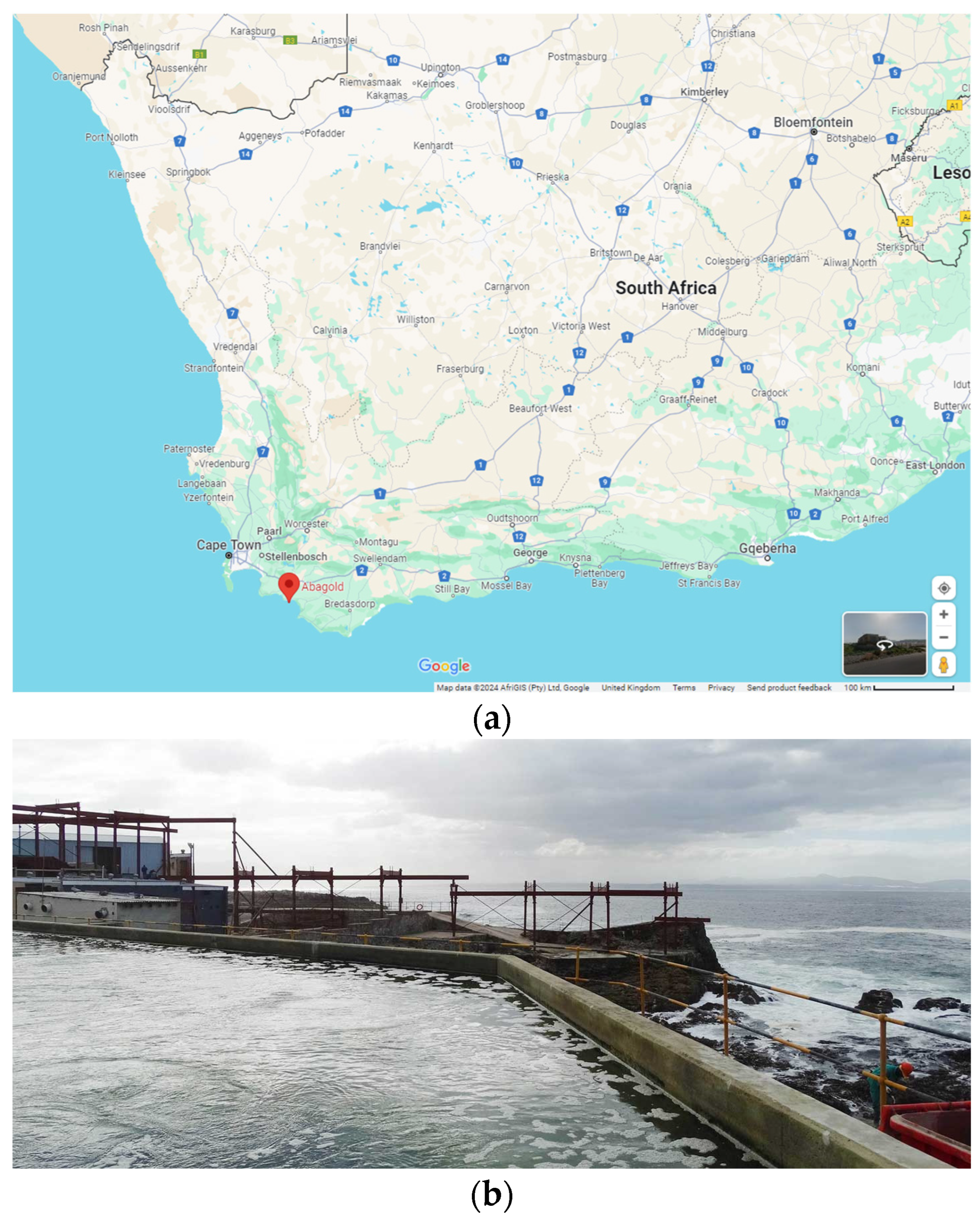
4.1. Data Collection Site

Abagold Limited (https://www.abagold.com/) cultivates the abalone species, Haliotis midae, a marine mollusc which is revered around the world as a food delicacy and is endemic to South Africa. Abagold exports live, canned, and dried abalone internationally via an integrated supply chain comprising a hatchery, four grow-out farms, and a processing factory, as well as a feed mill for sustainable feed supply and development. Abagold is located in Hermanus, nestled in Walker Bay, where pristine waters provide the necessary nutrients and environment to produce high-quality abalone (Figure 1).

4.2. Water Quality Parameter and Sensor Selection

Algal biomass dynamics are non-linear and non-stationary due to the complex interaction of physical, chemical, and biological parameters affecting the growth and accumulation of biomass, and this is a universal problem, so various models have been developed for its prediction; these are discussed in Section 2.2. Algae have unique pigments that they use for photosynthesis; these could be monitored by measuring chlorophyll-a, phycocyanin, and phycoerythrin. Chlorophyll-a has been used for many decades to monitor algal biomass [52]. The pigment phycocyanin is a more specific indicator of blue-green algae in freshwater systems, and a similar pigment called phycoerythrin is a useful indicator of blue-green algae in marine systems [53]. In addition to these parameters, turbidity is also linked with the presence of algae in water. As the selected site uses water from the ocean, chlorophyll-a (named as CHL1 (470), for ease here), phycoerythrin (named as CHL2 (530) for ease here), and turbidity (Tb) were selected to monitor for HABs.

There are various sensors available on the market for these parameters; our selection was based on cost and ease of availability and delivery to the South African site.

Table 2. List of suitable sensor manufacturers.

Manufacturer/Instrument	Parameters	Distribution Point	Cost (GBP) (Only for Instrument)
In-situ, Inc. Aqua Troll 500	chlorophyll-a, phycoerythrin	South Africa	5109
Chelsea Technology Limited Trilux	chlorophyll-a, phycoerythrin and turbidity	United Kingdom	4070
Xylem EXO3	chlorophyll-a, phycoerythrin	South Africa	7500

lists three multi-parameter instruments that were short-listed as suitable candidates:

The main problem with the project was the long delivery times for the short-listed sensors; this was understood to be due to a global shortage (at the time, i.e., last year) of some components necessary for these instruments. The Trilux sensor was chosen as Chelsea Technology Limited (CTL) is a long-term project partner with the University of Bedfordshire, so CTL agreed to lend an instrument. All the data presented in this paper were collected using the Trilux sensor (Figure 2).

The parameters, chlorophyll-a (CHL1 (470)), phycoerythrin (CHL2 (530)), and turbidity (Tb), were measured in the units QSU, μg/L, and FNU, respectively (where QSU stands for quinine sulphate units and FNU stands for Formazin Nephelometric Unit). The phytoplankton data were recorded manually at fixed times for the months of January, February, and March. These months were chosen as this is the algal bloom peak time in South Africa as the sea temperatures are highest. Although the farm continues to monitor phytoplankton count throughout the year, this is usually very low during the other months of the year.

Trilux sensor measurements were recorded throughout the months of January, February, and March at 1 s intervals. However, the phytoplankton count was recorded at fixed times—usually in the morning at 7.40 a.m. Thus, to correlate with these data, Trilux measurements were averaged over a 20 s window for the corresponding date and time on which the phytoplankton count was recorded, as shown in

Table 3. Phytoplankton count and 20 sec averaged TriLux data from the Abagold farm.

Sample Number	Date	Time	CHL1(470) (QSU)	Tb (FNU)	CHL2(530)(μg/L)	Phytoplankton Count
2097	10 January 2023	07:40	587.36	913.18	668.46	2650
2100	11 January 2023	07:40	574.86	880.35	643.82	36,475
2102	11 January 2023	12:40	547.48	818.78	624.9	2450
2106	12 January 2023	07:40	564.97	833.26	645.07	40,900
2109	13 January 2023	10:00	519.94	761.65	644.01	7475
2111	16 January 2023	07:40	291.26	405.28	281.08	2725
2113	17 January 2023	07:40	204.49	270.24	172.56	225
2115	18 January 2023	07:40	160.14	210.47	129.87	225
2117	19 January 2023	07:40	181.34	227.35	125.72	200
2119	20 January 2023	07:40	133.3	192.19	110.42	125
2122	23 January 2023	07:58	122.24	244.26	153.84	225
2124	24 January 2023	07:40	76.94	149.72	107.45	725
2127	25 January 2023	07:40	111.14	211.9	163.76	425
2129	26 January 2023	07:40	139.19	278.49	221.26	1700
2131	27 January 2023	07:40	124.53	250.56	196.03	3150
2133	30 January 2023	07:40	169.16	289.41	200.6	75
2135	31 January 2023	07:40	170.37	286.01	204.91	950
2137	1 February 2023	07:40	181.9	306.23	224.78	150
2139	2 February 2023	07:40	209.94	353.66	238.66	725
2141	3 February 2023	07:40	185.23	333.7	243.69	2225
2143	6 February 2023	07:40	193.37	361.69	295.29	925
2145	7 February 2023	07:40	249.15	360.36	269.27	925
2147	8 February 2023	07:40	252.34	406.9	302.79	375
2149	9 February 2023	07:40	359.09	611.48	468.39	1200
2151	10 February 2023	07:40	273.59	377.57	281.56	800
2153	13 February 2023	07:40	408.62	508.17	390.5	675
2160	17 February 2023	07:40	331.44	627.11	632.65	7475
2162	20 February 2023	07:40	96.68	174.63	112.45	250
2164	21 February 2023	07:40	141.96	186.75	99.63	575
2166	22 February 2023	07:40	168.93	211.61	111.27	475
2168	23 February 2023	07:40	102.61	149.74	93.1	1650
2170	24 February 2023	07:40	102.34	155.05	98.27	1200
2172	27 February 2023	07:40	201.81	241.64	128.54	575
2174	28 February 2023	07:40	275.05	312.1	155.98	750
2176	1 February 2023	07:40	333.6	330.24	157.46	750
2178	2 February 2023	07:40	464.66	429.99	200.13	925
2181	6 February 3023	07:40	904.28	1000	708.17	300
2183	7 February 2023	07:40	632.79	799.17	470.68	200

below and plotted in Figure 3. Phytoplankton counts are only measured at specific times, so these are indicated as dots on the graph, whereas other parameters are measured continuously, represented with line diagrams.

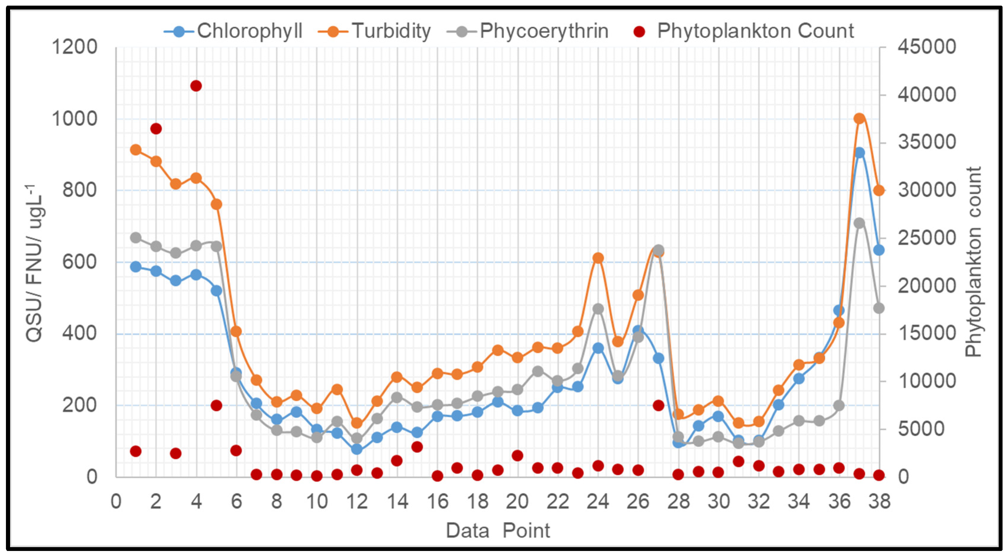
5. Statistical Analysis

Trilux sensor measurements were recorded throughout the months of January, February, and March. These measurements were processed, as described in Section 4.2, and are presented in Table 3 together with the phytoplankton count measured each day. Phytoplankton count is representative of algal biomass, so although it is not actually measuring specific HABs, the expectation is that a higher phytoplankton count would imply a higher probability of an HAB. The TriLux data presented in Table 3 were already cleaned and pre-processed. Pre-processing involved interpolating any missing data points; this was carried out before taking a 20 s window average. The next step was to conduct a statistical analysis of the collected data to establish correlation. The results presented here used Microsoft Office Excel 365 2016, statistics, and a data analysis toolbox. In addition, MATLAB 14 was used for data filling and cleaning.

Pearson’s correlation [54] coefficient technique is used to explore the correlation between the sensor parameters—chlorophyll, phycoerythrin, and turbidity—and the phytoplankton data. The Pearson correlation coefficient between two variables, X and Y, is formally defined as the covariance of the two variables divided by the product of their standard deviations (which acts as a normalisation factor), and it can be equivalently defined by

$${\mathrm{r}}_{\mathrm{xy}}=\frac{\sum (x_i-\overline{x})\sum (y_i-\overline{y})}{\sqrt{{\sum (x_i-\overline{x})}^2}\sqrt{{\sum (y_i-\overline{y})}^2}}$$

(1)

where $\overline{x}$ = $\frac{1}{n}{\sum }_{i=1}^N{x}_i$ denotes the mean of x and $\overline{y}$ = $\frac{1}{n}{\sum }_{i=1}^N{y}_i$ denotes the mean of y. The coefficient r_xy ranges from −1 to 1 and is invariant on linear transformations of either variable.

The table below shows the correlations obtained between the measured chlorophyll-a (CHL1 (470)), phycoerythrin (CHL2 (530)), turbidity, and phytoplankton data.

Table 4. Correlation table for TriLux data and phytoplankton count from Abagold Sea View farm.

	Chlorophyll (CHL1 (470))	Turbidity	Phycoerythrin (CHL2 (530))	Phytoplankton
Chlorophyll (CHL1 (470))	1	0.9489	0.8706	0.3858
Turbidity		1	0.9716	0.4854
Phycoerythrin (CHL2 (530))			1	0.5094
Phytoplankton				1

shows a strong positive correlation between the sensor parameters and the phytoplankton count. The next step is to develop a regression equation using regression analysis. For the regression analysis, phytoplankton data are the dependent variable and CHL1 (470), CHL2 (530), and turbidity are chosen as independent variables.

The regression analysis of the data in Table 3 gives the following equation:

Phytoplankton = −3596 − 30.18 CHL1 + 35.59 Tb + 4.613 CHL2

(2)

This equation forms the foundation to predict harmful algal blooms, using an artificial neural network (ANN) forecasting model as described in [38]. The HAB/phytoplankton forecasting model would be an extension of that developed in [38] as it involves three independent variables to predict one dependent variable. The hybrid forecasting model method used merges the ensemble empirical mode decomposition (EEMD) method, a deep learning long-short term memory (LSTM) neural network (NN), and the multivariate linear regression (MLR) method [55,56,57]. The ANN model that we developed for reliably forecasting algal biomass is described in [58]. The model would be further strengthened with more data collected over different HAB periods. The final intention is to give at least half a day’s warning to the business in addition to their continuous access to chlorophyll data. This forms an essential part of their sophisticated risk model which also considers environmental conditions like temperature differential, wind speed and direction, and animal behaviour to determine the likelihood of HABs.

6. Forecasting Advantages and Challenges

The mathematical model developed [38] shows that early forecasting of harmful phytoplankton (algal blooms) using in situ-measured chlorophyll-a (470), turbidity, and phycoerythrin (530) is possible; this forecasting capability will undeniably prove to be a useful tool for the aquaculture industry. The data in Table 3 show the phytoplankton count at the initial entry point of water into the farm. Other locations are also monitored, but as the intention here was to demonstrate the correlation with chlorophyll data collected using sensors, those measurements are not reported here. In this case study, the methodology described to deliver early forecasting of HABs in commercial abalone production has been demonstrated. This approach should be transferable to other aquaculture systems; however, the toxicity thresholds will need to be determined and verified for a specific production environment and product. It is important to emphasise that the sensor measurements here relate to algal biomass and the resulting early warning system would be a useful tool to avert a bloom. For example, the 2017 bloom in South Africa occurred within an afternoon and stayed in the bay for weeks.

6.1. Advantages

This early warning system will allow farms like Abagold to mitigate the impact of eventualities like an HAB more effectively and efficiently. Subsequently, this reduces risk and ensures the long-term sustainability of the company, whilst safeguarding a significant employer in the local community. This model can complement other existing processes that Abagold already has in place. For example, Abagold uses a risk model to determine the probability of an HAB occurring. If the probability is high, then the farm is on high alert and employs additional mitigation measures, including increased sampling.

The main advantage of developing a forecasting model would be to give farms like Abagold an early warning of upcoming blooms, a tool that can assign a risk category with a level of prediction, which will enable action to be taken by the farm to minimise negative impacts of blooms. A system such as this will safeguard the aquaculture industry in South Africa, particularly in the Walker Bay region, where Abagold is based. Early warning allows farms to take remedial actions which include recirculating their water (i.e., blocking incoming water from the ocean), repeated water/abalone sampling, and pre-emptive harvesting.

Additionally, there are significant benefits to remote monitoring, without the need to be present on site. It allows for continuous risk management (including in the evenings and at weekends) and the development of a historical reference database to better understand changes over time.

6.2. Challenges

One of the main challenges in developing an HAB forecasting model is acquiring access to reliable data. Once a model is developed and established with repeated training and testing, it can be deployed for use with live data. However, during the development of the model, we still need to rely on manual phytoplankton counting, which could be prone to errors. The Trilux sensor is a fluorescence-based optical sensor and needs to be kept clean as it is prone to debris depositing on the water-exposed optical surface. Abagold, however, has a process of ensuring that the sensors are cleaned regularly by a dedicated diver. So, the data quality is ensured.

Although this is a ‘low’-cost system, it still requires a capital investment from the business. Abagold is a prominent member of the Abalone Farmers Association of South Africa (AFASA), which represents the abalone producers in South Africa (of which there are 14), an industry which provides employment for some 2000 individuals. There is the opportunity to disseminate the work completed here through this association to deliver broader impacts across the sector and region. The model could additionally have further applications in the future, including in the mussel, oyster, and finfish aquaculture industry in South Africa, as well as applications for recreational coastal users.

This project illustrated a need for training in the sector; this is essential not only for developing useful skills among the workforce but also in challenging mindsets through, as an example, digital and technical literacy campaigns. Reservations regarding digital technologies amongst the general workforce include the replacement of manual jobs. However, appropriately implemented digital technologies stand to allow for improved effectiveness and efficiency, whilst upskilling critical workforces.

7. Conclusions and Further Work

This article presents the development of a novel hybrid water quality forecasting model based on a TriLux multi-parameter sensor to monitor water quality parameters and the application of a specialised EEMD method, with a deep learning LSTM NN. The actual experimental real water quality data from Abagold Limited show a good correlation as a basis for the forecasting model.

The mathematical model developed so far shows that early forecasting of phytoplankton activity with the aid of the actual sensor-monitored chlorophyll-a (470), turbidity, and phycoerythrin (530) time-series data is possible. This forecasting will undeniably prove to be a useful tool in the management of HABs in the aquaculture industry.

Early prediction of HABs will ensure a reduction in animal health issues whilst improving economic turnover for the aquaculture sector. Furthermore, some HAB-associated species are also detrimental to human health. Early detection allows for improved food safety and export compliance. There is a confirmed correlation between monitoring parameters like chlorophyll and turbidity with phytoplankton count. In seeking solutions to the aforementioned challenges associated with prevailing water quality monitoring in the aquaculture industry, more research must be carried out in areas of effectiveness, efficiency, prediction accuracy, reliability, and the application of existing water quality prediction models and management methodologies in the precision aquaculture ecosystem.

References

1. Hallegraeff, G.M. Harmful Algal Blooms: A Global Overview. In Manual on Harmful Marine Microalgae; UNESCO Publishing: Paris, France, 2003; Volume 33, pp. 1–22. [Google Scholar]
2. Grattan, L.M.; Holobaugh, S.; Morris, J.G. Harmful algal blooms and public health. Harmful Algae 2016, 57 Pt B, 2–8. [Google Scholar] [CrossRef]
3. Costa, P.R.; Pereira, P.; Guilherme, S.; Barata, M.; Nicolau, L.; Santos, M.A.; Pacheco, M.; Pousão-Ferreira, P. Biotransformation modulation and genotoxicity in white seabream upon exposure to paralytic shellfish toxins produced by Gymnodinium catenatum. Aquat. Toxicol. 2012, 106–107, 42–47. [Google Scholar] [CrossRef] [PubMed]
4. Aguilera, A.; Gutiérrez, X.; Mayorga, J.; Villanueva, F.; Varela, D. Effects of Alexandrium catenella on Atlantic salmon post smolt. In Proceedings of the Abstract Book 17th International Conference on Harmful Algae, Florianopolis, Brazil, 9–14 October 2016; p. 145. [Google Scholar]
5. Díaz, P.A.; Álvarez, G.; Varela, D.; Pérez-Santos, I.; Díaz, M.; Molinet, C.; Seguel, M.; Aguilera-Belmonte, A.; Guzmán, L.; Uribe, E.; et al. Impacts of harmful algal blooms on the aquaculture industry: Chile as a case study. Perspect. Phycol. 2019, 6, 39–50. [Google Scholar] [CrossRef]
6. John, U.; Šupraha, L.; Gran-Stadniczeñko, S.; Bunse, C.; Cembella, A.; Eikrem, W.; Janouškovec, J.; Klemm, K.; Kühne, N.; Naustvoll, L.; et al. Spatial and biological oceanographic insights into the massive fish-killing bloom of the haptophyte Chrysochromulina leadbeateri in northern Norway. Harmful Algae 2022, 118, 102287. [Google Scholar] [CrossRef] [PubMed]
7. Brown, A.R.; Lilley, M.K.; Shutler, J.; Widdicombe, C.; Rooks, P.; McEvoy, A.; Torres, R.; Artioli, Y.; Rawle, G.; Homyard, J.; et al. Harmful Algal Blooms and their impacts on shellfish mariculture follow regionally distinct patterns of water circulation in the western English Channel during the 2018 heatwave. Harmful Algae 2021, 111, 102166. [Google Scholar] [CrossRef] [PubMed]
8. Matt, R. Algae Bloom Decimates Two B.C. Fish Farms. Vancouver Sun. 11 June 2018. Available online: https://vancouversun.com/news/local-news/algae-bloom-decimates-two-b-c-fish-farms (accessed on 14 March 2024).
9. Pitcher, G.C.; Foord, C.J.; Macey, B.M.; Mansfield, L.; Mouton, A.; Smith, M.E.; Osmond, S.J.; van der Molen, L. Devastating farmed abalone mortalities attributed to yessotoxin-producing dinoflagellates. Harmful Algae 2019, 81, 30–41. [Google Scholar] [CrossRef] [PubMed]
10. Anderson Donald, M.; Jack, R. Harmful Algal Blooms. Assessing Chile’s Historic HAB Events of 2016. Available online: https://www.globalseafood.org/wp-content/uploads/2017/05/Final-Chile-report.pdf (accessed on 14 March 2024).
11. Martino, S.; Gianella, F.; Davidson, K. An approach for evaluating the economic impacts of harmful algal blooms: The effects of blooms of toxic Dinophysis spp. on the productivity of Scottish shellfish farms. Harmful Algae 2020, 99, 101912. [Google Scholar] [CrossRef] [PubMed]
12. Campbell, A.; Hudson, D.; Mcleod, C.; Nicholls, C.; Pointon, A. Tactical Research Fund: Review of the 2012 Paralytic Shellfish Toxin Event in Tasmania Associated with the Dinoflagellate Alga, Alexandrium tamarense; FRDC Project 2012/060; SafeFish: Adelaide, Australia, 2013. [Google Scholar]
13. Trainer, V.L.; Yoshida, T. (Eds.) Proceedings of the Workshop on Economic Impacts of Harmful Algal Blooms on Fisheries and Aquaculture; PICES Sci. Rep. No. 47; North Pacific Marine Science Organization (PICES): Honolulu, HI, USA, 2014; 85p. [Google Scholar]
14. Rodríguez, G.R.; Villasante, S.; García-Negro, M.D.C. Are red tides affecting economically the commercialization of the Galician (NW Spain) mussel farming? Mar. Policy 2011, 35, 252–257. [Google Scholar] [CrossRef]
15. Pitcher, G.C.; Louw, D.C. Harmful algal blooms of the Benguela eastern boundary upwelling system. Harmful Algae 2021, 102, 101898. [Google Scholar] [CrossRef]
16. Pitcher, G.; Franco, J.; Doucette, G.; Powell, C.; Mouton, A. Paralytic shellfish poisoning in the abalone Haliotis midae on the west coast of South Africa. J. Shellfish. Res. 2001, 20, 895–904. [Google Scholar]
17. Treasurer, J.W.; Hannah, F.; Cox, D. Impact of a phytoplankton bloom on mortalities and feeding response of farmed Atlantic salmon, Salmo salar, in west Scotland. Aquaculture 2003, 218, 103–113. [Google Scholar] [CrossRef]
18. Dale, B.; Edwards, M.; Reid, P.C. Climate change and harmful algal blooms. In Ecology of Harmful Algae; Springer: Berlin/Heidelberg, Germany, 2006; pp. 367–378. [Google Scholar]
19. Gobler, C.J.; Doherty, O.M.; Hattenrath-Lehmann, T.K.; Griffith, A.W.; Kang, Y.; Litaker, R.W. Ocean warming since 1982 has expanded the niche of toxic algal blooms in the North Atlantic and North Pacific oceans. Proc. Natl. Acad. Sci. USA 2017, 114, 4975–4980. [Google Scholar] [CrossRef]
20. Gobler, C.J. Climate Change and Harmful Algal Blooms: Insights and perspective. Harmful Algae 2019, 91, 101731. [Google Scholar] [CrossRef]
21. Wells, M.L.; Trainer, V.L.; Smayda, T.J.; Karlson, B.S.; Trick, C.G.; Kudela, R.M.; Ishikawa, A.; Bernard, S.; Wulff, A.; Anderson, D.M.; et al. Harmful algal blooms and climate change: Learning from the past and present to forecast the future. Harmful Algae 2015, 49, 68–93. [Google Scholar] [CrossRef]
22. Bondur, V.; Zamshin, V.; Chvertkova, O.; Matrosova, E.; Khodaeva, V. Detection and Analysis of the Causes of Intensive Harmful Algal Bloom in Kamchatka Based on Satellite Data. J. Mar. Sci. Eng. 2021, 9, 1092. [Google Scholar] [CrossRef]
23. Bu, X.; Liu, K.; Liu, J.; Ding, Y. A Harmful Algal Bloom Detection Model Combining Moderate Resolution Imaging Spectroradiometer Multi-Factor and Meteorological Heterogeneous Data. Sustainability 2023, 15, 15386. [Google Scholar] [CrossRef]
24. Luis, K.; Köhler, P.; Frankenberg, C.; Gierach, M. First light demonstration of red solar induced fluorescence for harmful algal bloom monitoring. Geophys. Res. Lett. 2023, 50, e2022GL101715. [Google Scholar] [CrossRef]
25. Jordan, T.M.; Simis, S.G.H.; Grötsch, P.M.M.; Wood, J. Incorporating a Hyperspectral Direct-Diffuse Pyranometer in an Above-Water Reflectance Algorithm. Remote. Sens. 2022, 14, 2491. [Google Scholar] [CrossRef]
26. Wu, D.; Li, R.; Zhang, F.; Liu, J. A review on drone-based harmful algae blooms monitoring. Environ. Monit. Assess. 2019, 191, 211. [Google Scholar] [CrossRef]
27. Horricks, R.A.; Bannister, C.; Lewis-McCrea, L.M.; Hicks, J.; Watson, K.; Reid, G.K. Comparison of drone and vessel-based collection of microbiological water samples in marine environments. Environ. Monit. Assess. 2022, 194, 439. [Google Scholar] [CrossRef]
28. Graham, C.T.; O’Connor, I.; Broderick, L.; Broderick, M.; Jensen, O.; Lally, H.T. Drones can reliably, accurately and with high levels of precision, collect large volume water samples and physio-chemical data from lakes. Sci. Total. Environ. 2022, 824, 153875. [Google Scholar] [CrossRef]
29. Koparan, C.; Koc, A.B.; Privette, C.V.; Sawyer, C.B. In Situ Water Quality Measurements Using an Unmanned Aerial Vehicle (UAV) System. Water 2018, 10, 264. [Google Scholar] [CrossRef]
30. Castendyk, D.; Voorhis, J.; Kucera, B. A Validated Method for Pit Lake Water Sampling Using Aerial Drones and Sampling Devices. Mine Water Environ. 2020, 39, 440–454. [Google Scholar] [CrossRef]
31. Secchi, A. Reports on Experiments made on board the Papal Steam Sloop L’lmmacolata Concezione to determine the transparency of the sea. In Sul Moto Ondoso del Mare e su le Correnti di esso Specialmente su Quelle Littorali, 2nd ed.; ON1 Transl. A-655, Op-923 M4B; Department of the Navy, Office of Chief of Naval Operations: Rome, Italy, 1866; pp. 258–288. (In Italian) [Google Scholar]
32. Holmes, R.W. The secchi disk in turbid coastal waters. Limnol. Oceanogr. 1970, 15, 688–694. [Google Scholar] [CrossRef]
33. Lee, Z.P.; Shang, S.; Hu, C.; Du, K.; Weidemann, A.; Hou, W.; Lin, J.; Lin, G. Secchi disk depth: A new theory and mechanistic model for underwater visibility. Remote Sens. Environ. 2015, 169, 139–149. [Google Scholar] [CrossRef]
34. Preisendorfer, R.W. Secchi disk science: Visual optics of natural waters. Limnol. Oceanogr. 1986, 31, 909–926. [Google Scholar] [CrossRef]
35. Boyce, D.G.; Lewis, M.R.; Worm, B. Global phytoplankton decline over the past century. Nature 2010, 466, 591–596. [Google Scholar] [CrossRef]
36. Brewin, R.J.W.; Brewin, T.G.; Phillips, J.; Rose, S.; Abdulaziz, A.; Wimmer, W.; Sathyendranath, S.; Platt, T. A Printable Device for Measuring Clarity and Colour in Lake and Nearshore Waters. Sensors 2019, 19, 936. [Google Scholar] [CrossRef]
37. MONOCLE Project—Multiscale Observation Networks for Optical Monitoring of Coastal Waters, Lakes and Estuaries (monocle-h2020.eu). Available online: https://monocle-h2020.eu/ (accessed on 31 December 2023).
38. Eze, E.; Kirby, S.; Attridge, J.; Ajmal, T. Time series chlorophyll—A concentration data analysis: A novel forecasting model for aquaculture industry. Eng. Proc. 2021, 5, 27. [Google Scholar] [CrossRef]
39. Low-Cost Instrument for Detection of Toxins in Seawater during Harmful Algal Blooms—Technology Partnerships Office. Available online: https://techpartnerships.noaa.gov/low-cost-instrument-for-detection-of-toxins-in-seawater-during-harmful-algal-blooms/ (accessed on 4 January 2024).
40. Flow Cam FlowCam|Flow Imaging Analysis for the Life Sciences. Available online: https://www.fluidimaging.com (accessed on 4 January 2024).
41. Barrowman, P.; Adams, H.; Southard, M.; Davis, J.; Parkhurst, M.; Webb, J.; Lee, H. Establish Trigger Levels for Harmful Algal Blooms. Opflow 2023, 49, 12–16. [Google Scholar] [CrossRef]
42. Babin, M.; Roesler, C.S.; Cullen, J.J. (Eds.) Real-Time Coastal Observing Systems for Marine Ecosystem Dynamics and Harmful Algal Blooms: Theory, Instrumentation and Modelling; Oceanographic Methodology Series; UNESCO: Paris, France, 2008; 860p. [Google Scholar] [CrossRef]
43. Ralston, D.K.; Moore, S.K. Modeling harmful algal blooms in a changing climate. Harmful Algae 2020, 91, 101729. [Google Scholar] [CrossRef]
44. Litchman, E. Understanding and predicting harmful algal blooms in a changing climate: A trait-based framework. Limnol. Oceanogr. Lett. 2022, 8, 229–246. [Google Scholar] [CrossRef]
45. Lee, S.; Lee, D. Improved Prediction of Harmful Algal Blooms in Four Major South Korea’s Rivers Using Deep Learning Models. Int. J. Environ. Res. Public Health 2018, 15, 1322. [Google Scholar] [CrossRef]
46. Qin, Q.; Shen, J.; Reece, K.S.; Mulholland, M.R. Developing a 3D mechanistic model for examining factors contributing to harmful blooms of Margalefidinium polykrikoides in a temperate estuary. Harmful Algae 2021, 105, 102055. [Google Scholar] [CrossRef]
47. Kim, J.; Lee, T.; Seo, D. Algal bloom prediction of the lower Han River, Korea using the EFDC hydrodynamic and water quality model. Ecol. Model. 2017, 366, 27–36. [Google Scholar] [CrossRef]
48. Yu, P.; Gao, R.; Zhang, D.; Liu, Z.-P. Predicting coastal algal blooms with environmental factors by machine learning methods. Ecol. Indic. 2021, 123, 107334. [Google Scholar] [CrossRef]
49. Sustainable Aquaculture Innovation Centre (SAIC) Project. Available online: https://www.sustainableaquaculture.com/projects/project-list/real-time-modelling-and-prediction-of-harmful-algal-blooms/ (accessed on 14 January 2024).
50. South Africa National OCIMS. Available online: https://ocims-dev.dhcp.meraka.csir.co.za/ (accessed on 14 January 2024).
51. Strategic Environmental Assessment for Marine and Freshwater Aquaculture Development in South Africa; CSIR Report Number CSIR/IU/021MH/ER/2019/0050/A; Department of Environment, Forestry and Fisheries: Stellenbosch, South Africa, 2019; ISBN 978-0-7988-5646-1.
52. Chapman, D.J.; Chapman, V.J. The Algae; Springer: Berlin/Heidelberg, Germany, 1973. [Google Scholar]
53. Monitoring Algal Blooms. Available online: https://chelsea.co.uk/monitoring-algal-blooms-maintaining-water-quality-and-chelsea-technologies-solutions-for-commercial-aquaculture/ (accessed on 21 December 2023).
54. Razi, M.A.; Athappilly, K. A comparative predictive analysis of neural networks (NNs), nonlinear regression and classification and regression tree (CART) models. Expert Syst. Appl. 2005, 29, 65–74. [Google Scholar] [CrossRef]
55. Abyaneh, H.Z. Evaluation of multivariate linear regression and artificial neural networks in prediction of water quality parameters. J. Environ. Health Sci. Eng. 2014, 12, 40. [Google Scholar] [CrossRef]
56. Wu, Z.; Huang, N.E. Ensemble empirical mode decomposition: A noise-assisted data analysis method. Adv. Adapt. Data Anal. 2009, 1, 1–41. [Google Scholar] [CrossRef]
57. Brownlee, J. Stacked Long Short-Term Memory Networks Develop Sequence Prediction Models in Keras. 14 August 2019. Available online: https://machinelearningmastery.com/stacked-long-short-term-memory-networks/ (accessed on 19 February 2021).
58. Eze, E.; Kirby, S.; Attridge, J.; Ajmal, T. Aquaculture 4.0: Hybrid neural network multivariate water quality parameters forecasting model. Sci. Rep. 2023, 13, 16129. [Google Scholar] [CrossRef]
Figure 1. Data collection site: (a) location of Abagold Farm and (b) primary sump, Abagold Sea View Farm.
Sustainability 16 03650 g001
Figure 2. Installation of Chelsea Technology Limited Trilux sensor at Abagold. (a) Chealsea TriLux, (b) TriLux installed at Abagold and (c) data console for TriLux.
Sustainability 16 03650 g002
Figure 3. Plot for measured parameters from Table 3.
Sustainability 16 03650 g003