Article

Optimization Based on Computational Fluid Dynamics and Machine Learning for the Performance of Diffuser-Augmented Wind Turbines with Inlet Shrouds

Department of Aerospace and Systems Engineering, Feng Chia University, Taichung 407102, Taiwan
*
Author to whom correspondence should be addressed.
Sustainability 2024, 16(9), 3648; https://0-doi-org.brum.beds.ac.uk/10.3390/su16093648
Submission received: 29 February 2024 / Revised: 18 April 2024 / Accepted: 19 April 2024 / Published: 26 April 2024
(This article belongs to the Special Issue Application of Green Energy Technology in Sustainable Environment)

Abstract

:
A methodology that could reduce computational cost and time, combining computational fluid dynamics (CFD) simulations, neural networks, and genetic algorithms to determine a diffuser-augmented wind turbine (DAWT) design is proposed. The specific approach used implements a CFD simulation validated with experimental data, and key parameters are analyzed to generate datasets for the relevant mathematical model established with the backpropagation neural network algorithm. Then, the mathematical model is used with the non-dominant sorting genetic algorithm II to optimize the design and improve the DAWT design to overcome negative constraints such as noise and low energy density. The key parameters adopted are the diffuser’s flange height/angle, the diffuser’s length, and the rotor’s axial position. It was found that the impact of the rotor’s axial position on the power output of the DAWT is the most significant parameter, and a well-designed diffuser requires accelerating the airflow while maintaining high-pressure recovery. Introducing a diffuser can suppress the wind turbine’s noise, but if the induced tip vortex is too strong, it will have the opposite effect on the noise reduction.

1. Introduction

With the rapid increase in global energy demand and growing concerns for environmental sustainability, research on and application of renewable energy sources, e.g., solar, hydro, biomass, and wind energy [1,2], have become central issues in technology. The main advantage of renewable energy resources over conventional fossil resources involves the former’s significantly fewer environmental impacts (EIs), specifically during the operation phase [2]. However, relevant concerns should still be taken into account. For example, solar energy gained by using photovoltaic solar panels harnesses sunlight to generate electricity and is suitable for decentralized installations. Resource availability, land use requirements, and intermittency are often considered. Hydroelectric dams utilize flowing water to generate electricity and provide reliable baseload power. Concerns regarding EIs, such as habitat disruption and sedimentation, must be addressed. Biomass energy involves the combustion of organic materials such as wood or agricultural residues to produce heat or electricity. While biomass can be a renewable energy source, its sustainability depends on responsible forestry practices and the avoidance of competition with food production. Wind energy is generally regarded as a clean and sustainable source of electricity production. The potential EIs of wind turbine installations include wildlife habitat fragmentation; noise; visual and aesthetic pollution; the carbon footprint of its manufacture, transportation, and installation; and land use. Nevertheless, solar and wind energy are now competitive with conventional sources and command a high percentage of the investments in renewable power nowadays [3]. Additionally, from a techno-economic point of view, wind energy is the most mature form of renewable and clean energy [4].
Thus, wind energy has garnered extensive attention among these sources due to its wide availability and environmentally friendly attributes, which have emerged as pivotal drivers for energy transition [5,6,7]. For example, the total global installed capacity of wind turbines is 906 GW, and it shows nearly 9% growth, i.e., 77.6 GW in 2022, as reported by the Global Wind Energy Council (GWEC) in 2023 [6,7]. However, to fully unlock the potential of wind energy, numerous technological challenges must be addressed, and one such challenge lies in simultaneously enhancing the energy conversion efficiency of wind turbines while mitigating their impact on the environment, particularly concerning noise emissions [7,8,9]. As Nazir et al. [4] pointed out, noise pollution is the most critical impact of wind turbines on the environment. The wind turbines’ noise can be divided into two main types, i.e., aerodynamic and mechanical. Aerodynamic noise, the dominant one, is generated by airflow flowing through its components, e.g., the turbine blade, and produces a characteristic howling sound. Mechanical noise mainly comes from the generating equipment, such as the gearbox and linkages. Those noises can be minimized during the design phases of the blade, tower, and associated components [4,10].
Wind turbines can be principally classified into horizontal axis wind turbines (HAWTs) and vertical axis wind turbines (VAWTs), based on the orientation of the rotor’s rotational axis relative to the ground. The former has a rotor with a rotational axis parallel to the ground, while the latter’s is vertical. Generally speaking, HAWTs perform better at extracting wind power than do VAWTs; therefore, most commercial wind turbines are based on HAWTs [9]. When a diffuser is added to a HAWT, the resulting design is referred to as a diffuser-augmented wind turbine (DAWT), also known as a wind lens or shrouded wind turbine. The DAWT has a diffuser-type structure resembling a funnel, which can be modified by adding a broad-ring flange around the exit point (Figure 1). This design allows for the collection and concentration of the approaching wind, creating a wind-lens effect. Compared to traditional turbines, it has been proven that the DAWT can generate higher power given a specific turbine diameter and wind speed [11,12,13].
Consequently, the Levelized Cost of Energy (LCOE) for the unit may be reduced compared to an unshrouded generator if the cost of the diffuser is less than that of making a larger rotor to provide the equivalent power output [14,15]. Even if this technology is not significantly cheaper than non-ducted techniques, it still finds suitable niche applications, such as in the urban environment, due to its better suitability for smaller-scale applications [15,16]. A review article [17] highlights that conventional commercial wind turbines are typically designed to perform efficiently at high wind speeds, making them unsuitable for low-wind speed regions such as urban areas. Hence, it is necessary to enhance wind energy technology to make it suitable for low-wind speed regions [7]. The DAWT holds the potential to meet this demand, especially when utilizing small-scale wind turbines based on this design [18], and it offers a promising option for renewable energy generation, but requires careful design and implementation for optimal performance [16], so its improvement can become a topic worth studying.
Abe and Ohya [19] used numerical simulation methods to develop a small HAWT below 1.5 kW and employed a load instead of using the rotor effectiveness to analyze the flow field around a flanged diffuser. The geometric research parameters included flange height and diffuser opening angle. The results of the research show that avoiding the separation of the flow field in the diffuser and maintaining its high pressure–recovery coefficient tends to improve the performance of a wind turbine equipped with a flanged diffuser. Experiments and numerical simulations, a numerical approach similar to that used in Ref. [18], were employed by Abe et al. to analyze the flow field characteristics of the HAWT with/without a flanged diffuser [20]. After their research, they found that the flange diffuser will not only accelerate the approaching wind speed and thus increase the wind turbine’s power output, but also cause the rapid collapse of the blade tip vortex structure. They also showed that the computational results reasonably agree with the corresponding experimental data.
The velocity field of a HAWT with long and compact diffusers was measured using particle image velocimetry (PIV) to observe flow characteristics and flow acceleration phenomena [21]. Their study found that the flow field patterns were similar for both types of diffusers, and vortices behind the flange caused the flow acceleration phenomenon in both kinds. Ohya and Karasudani [14] experimentally measured and studied the power output of wind turbines with different flanged diffusers, also known as wind lenses, and conducted flow visualization observations. For the sake of practical application, considering the structure strength, they developed a compact-type flanged diffuser by evaluating different diffuser shapes, lengths, and heights. Their research revealed that the sectional shape of the diffuser with a cycloid curve exhibits the best performance, and that, under the same wind speed and wind turbine rotor diameter, employing wind-lens technology with proper geometric dimensions could increase the power of wind turbines by 2 to 3 times, compared to bare wind turbines. Flow visualization observations also showed that adopting wind lenses induces airflow acceleration, primarily due to low-pressure vortices arising behind the edges.
To find the influences of flange heights and lengths, Jafari and Kosasih [22] used numerical simulation to analyze the performance of wind turbines with simple frustum diffusers. Their results indicate the significant effects of these diffusers’ parameters on power augmentation, especially for the ratio of flange height to rotor diameter of 0.05–0.15. Additionally, flow separation inside the diffuser reduces power gain, which can be mitigated by increasing the length of the diffuser. Roshan et al. [23] used numerical simulation to explore the effects of using a stepped configuration on the diffuser duct of a DAWT and changing the relative position of the wind turbine rotor. The study’s results showed that placing the wind turbine rotor at the inlet section performs better, and implementing a stepped diffuser duct can increase the turbine’s efficiency in capturing energy from the wind. El-Zahaby et al. [24] used numerical simulation to explore the influence of the diffuser flange angle (θ) used in a DAWT. The results of their research showed that an optimal value for the flange angle (θ = 15°) can accelerate flow at the diffuser entrance, thereby increasing the generated power by 5%, compared to the one with θ = 0°. The research article by Ohya et al. [11] reported that wind lens technology can improve the quietness of wind turbines due to the cancellation of the blade tip vortex, reducing the noise. Review papers also pointed out that the shroud of the DAWT suppresses vortices generated from the turbine blades within the diffuser shroud, and consequently, it can enhance the aerodynamic performance [18,25] and decrease the noise of wind turbines [25]. In addition, adding a diffuser helps wind turbines to be applied in low-wind speed urban environments [16,26]. Heikal et al. [27] used numerical simulation to explore the effects of diffuser flange angle and inner flange depth on DAWT performance. The results of the research show that the effect of the flange angle will change with the tip speed ratio, and the impact of the inner flange depth is negative. They also concluded that the size and location of the vortex downstream of the diffuser flange significantly impact the power output of a DAWT.
The numerical study of Klistafani and Mukhsen [28] on DAWTs with various diffuser structures revealed that a curved diffuser provides better approaching wind flow acceleration than a flat diffuser due to more prominent vortices formed downstream. Numerical and experimental studies were carried out by Anbarsooz et al. [29] to analyze the maximum possible velocity increment of a flanged converging–diverging duct without considering the rotor. They revealed that adding a converging section to the flanged diffuser can enhance the approaching wind flow acceleration. Arifin et al. [30] numerically and experimentally studied the effects of changes in diffuser length and opening angle on a horizontal wind turbine. Their results showed that installing a diffuser with a specific length and opening angle can increase the generated power, resulting in values 1.6–2.1 times higher than one without a diffuser. Watanabe and Ohya [31] presented a simple theory that two performance coefficients, i.e., the flange’s back-pressure coefficient and the diffuser pressure recovery coefficient, can be used to predict the performance of DAWTs. They also indicated that the power output of the DAWT depends on the diffuser shape, length, and flange height.
The influences of rotor axial position, diffuser length, and opening angle on the power generation of DAWTs were numerically studied by Ramayee and Supradeepan [32]. Their parametric studies showed that the optimal diffuser opening angle is a function of its length, so it should not be fixed and has to be kept as a variable when changing the diffuser length. They also pointed out that the power output of a DAWT depends on the diffuser length and angle, rotor axial position, and tip clearance between the blade and diffuser duct. Hashem et al. [33] used a numerical approach to assess the effect of design parameters, including the diffuser shape, length, area ratio, and flange height, on power augmentation. Their results affirm that diffusers with a cycloidal profile and small length could perform better while maintaining large flange heights. Jauhar et al. [34] numerically performed a parametric study on the effects of diffuser opening angle, flange height, and rotor axial position on a DAWT. They indicated that the power output of the DAWT varies with its diffuser design and the resulting back pressure. Based on their results, it can be determined that a coupling effect exists among the parameters, and a proper combination is needed to achieve the best performance. Mutasher et al. [35] numerically conducted parametric studies, including diffuser opening angle, inlet nozzle length, and flange angle, to optimize the geometric dimensions of the converging–diverging duct without considering the rotor. Their results demonstrate a remarkable increase in the approaching wind speed by implementing the optimized diffuser and establish the necessity of adding an inlet shroud.
Noise emissions are one of the major issues for the wind turbine industry, especially for small-scale wind turbines, which are primarily installed in urban areas [36], where wind energy is a prominent alternative renewable energy source [37].
Aeroacoustic noise assessment for DAWTs was conducted numerically by Hashem et al. [38], work in which the Ffowcs-Williams–Hawkings (FW-H) equation and its integral solution were used to predict the noise radiating to the far field. The results indicated that the sound pressure level increases with increasing flange height, and a diffuser’s shape with a cycloid curve was recommended for less noise generation, a determination which was suggested to be computationally optimized by a genetic algorithm (GA) to reduce the noise emitted by small-scale application of DAWTs, making them more suitable for residential areas. It is worth mentioning that this study compared the noise emitted from the wind turbine with and without the diffuser and revealed that the DAWT generates higher noise intensity, a finding which is not consistent with the findings of other studies [11,25]. Lattice-Boltzmann Very-Large-Eddy Simulations (LB-VLES) were implemented for the solution of the flow field and the FW-H acoustic analogy was used for the far-field noise by Avallone et al. [39] to investigate the effects of varying tip clearance ratios on the aeroacoustics of a DAWT. They found that it strongly affects the far-field noise, which increases in smaller tip clearance ratio cases due to earlier flow separation along the suction side of the diffuser.
In recent years, the rapid advancements in computational fluid dynamics (CFD) and machine learning (ML) have presented novel opportunities for optimizing wind turbines. Applying CFD techniques to analyze the aerodynamics of wind turbines enables a deeper understanding of fluid dynamics within the wind field, thus enabling precise predictions of turbine performance [40,41]. Such a statement is evident from the review of the above papers, and it can be found that most of the above studies were conducted using computational fluid dynamics (CFD), such as Abe and Ohya [19], Abe et al. [20], Jafari and Kosasih [22], Roshan et al. [23], El-Zahaby et al. [24], Heikal et al. [27], Klistafani and Mukhsen [28], Anbarsooz et al. [29], Arifin et al. [30], Ramayee and Supradeepan [32], Hashem et al. [33], Jauhar et al. [34], Mutasher et al. [35], Hashem et al. [38], Avallone et al. [39], etc.; and the review paper by Agha et al. [42] also emphasized that CFD plays a vital role in the design and performance improvements of the DAWT. The reason is that CFD applications are increasingly widespread with the advancement of computer hardware. Meanwhile, experimental testing results are realistic but time-consuming, require costly investment, and are subject to experimental constraints. In contrast, CFD simulation is more time-efficient, with the advantages of cost-effectiveness and the ability to simulate various working conditions. Thus, CFD simulations and experimental measurements complement each other and have become indispensable tools for scientific research.
Concurrently, ML offers a more intelligent approach capable of autonomously learning patterns from extensive datasets to optimize control strategies and the operational efficiency of wind turbines [43,44]. Bin Abu Sofian et al. [45] mentioned that ML applications for wind energy generation are vital for sustainable energy production because ML is helpful in design, optimization, cost reduction, and, most importantly, improving wind energy’s efficacy, including advancing energy storage. Nikolić et al. [46] used the adaptive neuro-fuzzy (ANFIS) method with MATLAB/Simulink to estimate the impacts of diffusers on wind turbine performance. The data source used to train the ANFIS network was composed of CFD simulation results. Its input values included wind speed, number of blades, and presence of the diffuser; its output values include power coefficient, torque coefficient, and rotational speed of the rotor. The study results show that the predicted values are consistent with the experimental values, and the authors also suggest that other computing methods can be used to examine the same topic. Based on CFD simulation results, Liu et al. [47] used GA to optimize the diffuser profile to achieve velocity augmentation and drag reduction goals for DAWTs. The research procedure was to approximate the diffuser profile with a polynomial expression, use CFD to simulate the velocity augmentation and drag reduction, and then use GA to optimize the diffuser’s profile. Then, CFD calculation and GA operators are repeated until no better solutions are available. The results of their research show that the optimized diffuser can improve the velocity increase by 50% and reduce drag by 49%. In addition, this paper also mentions some simplification steps the research has taken, e.g., the CFD simulation was performed in a two-dimensional manner, and the outer boundary layers of the diffuser and the inner rotor blades are ignored.
Oka et al. [48] used the non-dominated sorting genetic algorithm II (NSGA-II) combined with a quasi-three-dimensional aerodynamic design method, including meridional viscous flow analysis and two-dimensional blade element designs, to optimize DAWT iteratively. The results of the research show that the optimized design’s power coefficient was significantly improved, after being verified by experiments and numerical simulations. It is worth mentioning that since the meridional viscous flow analysis cannot directly evaluate the power coefficient as the objective function, it was replaced by an equivalent parameter defined in this study. In combination with CFD simulation results, Khamlaj and Rumpfkeil [49] employed a multi-object genetic algorithm (MOGA) to simultaneously enhance power production, reduce drag, and increase thrust for DAWTs. This research utilized a piece-wise quadratic polynomial to define the diffuser shape, and the power, thrust, and drag coefficients were simulated by CFD. The rotor is modeled by incorporating the blade element method into the CFD approach to reduce the computational cost. The results of the research show that the proposed methodology can accurately predict the performance of DAWTs and achieve the optimization purposes. Leloudas et al. [50] used a two-dimensional CFD model with a differential evolution (DE) algorithm, assisted by artificial neural network meta-models, to optimize the DAWT diffuser. The procedure is implemented iteratively while the DE algorithm interacts with the parameterization (mesh deformation tool based on free-form deformation technique), CFD, and post-processing software. The objective function included the maximum average speed increase ratio without considering the rotor blades but considering geometric constraints and minimum resistance, and the results of the research show that the resulting designs can meet high-velocity acceleration and drag reduction requirements. A single-objective optimization design of DAWT with convergent–divergent ducts was conducted by Rahmatian et al. [51], who employed the response surface method (RSM) and GA incorporated with CFD for the study. In this research, 79 geometrical models defined using the design of experiments (DOE) were examined using CFD in the first step. Then, the simulated results were coupled with the RSM and GA to optimize the duct geometry with an objective function of maximum velocity at the duct throat. A HAWT was placed inside the optimal duct for performance evaluation in the second step. The results showed that the wind speed increases by 2.18 times, and the corresponding power coefficient increases by 3.94 times at the throat inside the optimized DAWT. In addition, this study indicated that the adding duct might break the vortices behind the turbine, reducing the noise level generated by the rotor. Shambira et al. [52] utilized RSM and a two-dimensional CFD model to develop and optimize the design of a DAWT equipped with a concentrator at the inlet without considering the rotor. The objective function was the throat velocity, and six geometrical parameters, including diffuser and concentrator angles and lengths, throat length, and flange height were considered in this research. This study utilized the central composite design to schedule 86 cases of different concentrator–diffuser geometrics for the CFD analysis, and RSM was employed to investigate the interactions of geometrical parameters and objective function by proposing a reduced quadratic model. It was found that the lengths of the concentrator and diffuser have the highest impacts on the throat velocity, and the optimized design displays a 1.953-fold increase in inlet wind speed at the throat position of the duct.
Based on the above literature review, the key points can be summarized as follows: 1. The DAWT is suitable for low-wind speed urban areas, and its technology is still worthy of further research [15,17,42]. 2. Compared with parametric studies on DAWTs, papers on its optimization study are relatively rare. 3. Research on combining CFD and ML for the DAWT is sparse. According to the literature reviewed in this study, Nikolić et al. [41], who employed the ML algorithm (ANFIS) to estimate the rotor performance of DAWT, did not conduct further optimization research and suggested trying other algorithms to examine the same topic. Optimization studies of DAWTs [47,48,49,50,51,52] all have their own compromised simplifications, mainly due to the high computational cost of CFD simulation. Therefore, for the sake of optimization, partial simplification is necessary. However, if an alternative approach could be adopted, i.e., using CFD simulation results to train ML algorithms to derive the corresponding mathematical model first and then incorporate it with the optimization algorithm, such a way could significantly reduce computational costs. 4. CFD, artificial neural network (ANN) algorithm, and genetic algorithm are reliable tools but rarely used together to study DAWTs. 4. The critical parameters of DAWT design include diffuser flange height/angle, diffuser profile/length/opening angle, rotor axial position/tip clearance, etc.. 5. Currently, there is a limited amount of research on the numerical simulation of DAWT noise, and the literature reviewed in this study indicates inconsistent assessments of this technology’s impact on noise.
According to the above summaries, this study intends to take small DAWTs suitable for urban area applications and with market potential as its research object, and develop a methodology that synergistically applies the CFD and ML techniques to simultaneously analyze and optimize the aerodynamic performance and noise characteristics and confirm its feasibility. We try to explore the augmentation of power output while minimizing noise generation during turbine operation. This endeavor contributes to enhancing the comprehensive utilization of wind energy and holds significant potential for mitigating the environmental impacts of wind power on surrounding areas.
This research reviews the current applications of CFD and ML techniques in wind turbine optimization, highlighting their integration potential. Subsequently, we introduce our chosen methods and optimization strategies, providing pertinent background knowledge. We then showcase optimization results based on CFD and ML techniques, offering detailed analyses of their effects and implications. Ultimately, we summarize the contributions of our research and discuss prospective directions for developing this interdisciplinary field. Based on the results obtained, we have confidence that our efforts can contribute to elevating the efficiency and sustainability of wind turbines, thus paving the way for a cleaner and more reliable energy supply.

2. Methodology

The research methods adopted in this study include CFD, ML algorithm—backpropagation neural network (BPNN), multi-objective genetic algorithm—NSGA-II, and experimental measurements. In this study, the reasons for selecting BPNN and NSGA-II as the implemented models can be described as follows:
  • BPNN algorithm: ML is a branch of artificial intelligence. In the modern era of software, ML depends on the prediction of datasets based on various algorithms for different software modules. A neural network is an ML model that implements a learning/training rule, i.e., when the input nodes are activated, synaptic weights are updated and forwarded to output nodes. Different training algorithms are available, like backpropagation, genetic, and krill herd algorithms [53]. The BPNN is such an ML model, one inspired by the biological neural network, and it is one of the oldest supervised-learning multilayer feed-forward neural network algorithms [54], having been proposed by Rumelhart, Hinton, and Williams in 1986 [55]. As introduced in the 1980s, it quickly became a focal point in neural network research due to its outstanding learning capability and adaptability [56]. Due to its backpropagating ability, it is highly suitable for problems with no relationships between the outputs and inputs [54]. Its flexibility, learning, and powerful fitting capabilities make it a robust tool for addressing complex problems [54,56]. Lillicrap et al. [57] pointed out that neural networks trained with backpropagation of error are at the heart of the recent successes of ML, including state-of-the-art speech and image recognition and language translation. In addition, backpropagation of error even underpins recent progress in unsupervised learning problems such as image and speech generation, language modeling, and other next-step prediction tasks. Over the years, BPNN has been proven to be the best algorithm among the multilayer perceptron algorithms [58]. Thus, the multilayer perceptron neural network trained with BPNN is the most popular and widely used network paradigm employed by engineering applications to solve practical problems, and it has demonstrated exceptional performance [53,54,56,59,60]. Inevitably, the traditional BPNN algorithm has some shortcomings, such as low convergence speed and an easy fall to the local minimum, but some remedies have been proposed to solve these problems [61]. In this study, the BPNN model is selected based on the abovementioned survey and then employed on the MATLAB platform, which will promptly update the latest modifications to the model.
  • NSGA-II algorithm: Inspired by Darwin’s theory of species evolution, John Holland proposed the genetic algorithm (GA) in 1975, which is widely used in various fields, including artificial intelligence, logistics distribution, and engineering science applications. It can be employed as an optimization algorithm that simulates the biological evolution process for multi-objective optimization problems (MOPs) [62]. In the real world, it is challenging to determine optimal solutions over MOPs with multiple conflicting objectives in complex systems. In such a situation, it is impossible to compute a single optimal solution. Therefore, the most common solution concept is to compute a set of Pareto optima, solutions that cannot be improved in one objective without accepting a worsening in others, and then let a decision-maker select the final solution based on their preference [63]. As a mainstream method for solving MOPs, the development and application of evolutionary algorithms (EAs) has attracted thousands of researchers since the 1950s [64]. EAs profit from their general ability to work with sets of solutions, are the standard approach to MOPs, and have many successful applications [63]. The NSGA-II algorithm, a model initially proposed by Deb et al. [65] in 2002, is considered the most prominent multi-objective EA [63,66] with the most popular GA framework [64], and has served as a powerful decision-space exploration engine, based on GA, used to solve MOPs [67]. So far, it has been cited more than 50,000 times on Google Scholar [68] and is becoming one of the most widely used algorithms for solving MOPs in various applications in different fields [12,68,69,70]. It has been verified that the Pareto frontier obtained by the NSGA-II algorithm is evenly distributed and has good convergence and robustness. [71]. We take advantage of its high competence, efficiency, and strength in dealing with most MOPs and adopt it in this research.
Firstly, based on the bare wind turbine (BWT) experimental results presented in the literature [72], CFD numerical simulation validation is carried out, and then the Taguchi orthogonal array [73] is implemented for planning the design parameters (flange height/angle, diffuser length, and rotor axial position, as shown in Figure 1), before proceeding to the numerical simulations. The obtained simulation datasets are used as the training, validation, and testing data of the BPNN to establish a predictive mathematical model (the input values are the design parameter conditions, the output values are the objective functions, i.e., the power and noise generated by the wind turbine), and finally will be used with the NSGA-II algorithm, which takes the BPNN mathematical model as its fitness function, to optimize the design of the DAWT to obtain the optimal combination of each parameter. This research will then construct the solid model and conduct numerical simulations based on the obtained optimized combinations by comparison and analysis with the selected performance evaluation indicators (generated power/noise value) and flow/acoustic characteristics. Finally, 3D printing will be employed to produce a scaled-down model of the optimized DAWT configurations for qualitative experimental testing to confirm their effectiveness. The research flowchart is shown in Figure 2, and the details of each method are described as follows:

2.1. Computational Fluid Dynamics (CFD)

This research employs the CFD software ANSYS Fluent 2023 R2 to study the three-dimensional flow and acoustic fields. In this study, the SST k-ω turbulence model is used as a closure for the Reynolds-averaged Navier–Stokes (RANS) equations, for this model accounts for turbulent shear stress transport, exhibits good performance in near-wall boundary layers [35], and is reliable in predicting flow separation under adverse pressure gradients [34]. Thus, it gains a broad consensus as to its suitability for wind turbine applications [23,27,28,29,30,31,32,33,35]. For aeroacoustic simulation, the Ffowcs-Williams–Hawkings (FW-H) formulation is adopted, as it is the most general form of Lighthill’s acoustic analogy and is capable of predicting sound generated by equivalent acoustic sources such as dipoles and quadrupoles of the far-field noise, and then is commonly used to simulate the aeroacoustic noise emitted from shrouded wind turbines [38,39]. The governing equations, including the RANS equations, SST k-ω turbulence model [74], FW-H equation [75], and broadband noise source models [76,77], used for these simulations are listed as follows:
ρ t + x i ρ u i = 0
t ρ u i + x j ρ u i u j = ρ g i p x i + x j μ u i x j + u j x i 2 3 δ i j u l x l + x j ρ u i u i ¯
where δ i j = 0   if   i j 1   if   i = j , u i = u ¯ i + u , u i is the velocity component, u ¯ i is the average velocity, u is the velocity fluctuation, μ is the dynamic viscosity, ρ is the density, p is the pressure, ρ u v ¯ is the Reynolds Stress, based on the Boussinesq assumption ρ u i   u j ¯ = μ t u i x j + u j x i 2 3 ρ k + μ t u l x l δ i j , and μ t = ρ k ω is the turbulent viscosity that can be obtained through solving the following k-ω equations.
t ρ k + x j ρ k u j = x j μ + μ t σ k k x j ρ u i   u j ¯ u j x i ρ β f β k ω
t ρ ω + x j ρ ω u j = x j μ + μ t σ ω ω x j ω k ρ u i   u j ¯ u j x i ρ β f B ω 2
where β = β i 1 + 1.5 F M t , f β = 1       χ k 0 1 + 680 χ k 2 1 + 400 χ k 2 χ k > 0 , χ k = 1 ω 3 k x j ω x j , χ ω = Ω i j Ω j k S k i 0.09 ω 3 , β = 0.072 1 1.5 β i 0.072 F M t , f β = 1 + 70 χ w 1 + 80 χ w , β   i = 0.09 4 / 15 + Re t / 8 4 1 + Re t / 8 4 , Re t = ρ k μ ω , M t 2 = 2 k γ R T , F M t = 0        M t 0.25 M t 2 0.25 2 M t > 0.25 , Ω i j = 1 2 u i x j u j x i , and S i j = 1 2 u i x j + u j x i .
1 a 0 2 p t 2 2 p = 2 x i x j T i j H f x i P i j n j + ρ u i u n v n δ f + t ρ 0 v n + ρ u n v n δ f
where T i j = ρ u i u j + P i j a 0 2 ρ ρ 0 δ i j is the Lighthill stress tensor, H(f) is the Heaviside function, P i j = p δ i j μ u i x j + u j x i 2 3 u k x k δ i j is the compressive stress tensor, un is the velocity component normal to the surface, vi is the surface velocity component, vn is the surface velocity component normal to the surface, a0 is the far-field sound speed, δ(f) is the Dirac delta function, and p′ is the sound pressure at the far field (p= p − p0).
P A = α ρ 0 u 3 l u 5 a 0 5 = α ε ρ 0 ε M t 5 ,   M t = 2 k a 0
P A = 1 ρ 0 a 0 0 2 π 0 π p 2 ¯ r 2 sin θ d θ d ψ = S I y d S y
where αε = 0.1, I y = A c y 12 ρ 0 π a 0 3 p t 2 ¯ . Equation (6) is Proudman’s formula, which indicates the quadrupole source strength related to turbulent shear stress and can be used to calculate the acoustic power. Equation (7) is the boundary layer noise source model, which can simulate the dipole source strength related to pressure fluctuations and can be used to calculate the acoustic surface power.
Regarding numerical methods, Fluent’s solver uses a finite-volume-based technique, and the governing equations with appropriate boundary and initial conditions are converted into a system of algebraic equations and solved numerically by the algebraic multigrid solver. The convection and diffusion terms of the governing equations are all calculated using the second-order upwind and central difference schemes, respectively, to ensure calculation accuracy, and the coupling between pressure and velocity is achieved using the coupled algorithm.

2.2. Backpropagation Neural Network (BPNN)

The BPNN is a supervised learning algorithm that can achieve the desired target output value by continuously adjusting the weights and biases of the network based on the error between the predicted output and actual output. Its architecture is shown in Figure 3, in which the network structure consists of input, hidden, and output layers, and it optimizes weights through the backpropagation algorithm, i.e., it learns by calculating the output layer’s errors to find the hidden layers’ errors.
The neurons in the hidden layer of BPNN can be expressed as n e t j = f i = 1 I w i j × n e t i , and the neurons in the output layer can be expressed as n e t k = f j = 1 J w j k × n e t j , where f is the activation function, and the Sigmoid function f x = 1 1 + e x is generally selected. This function can transform any value in the domain to a number between 0 and 1, net is the neuron, and wij is the weight between neurons i and j. BPNN uses the least-squares method for weight adjustment, and its process is as follows: 1. randomly initialize the weights; 2. use the current weights to calculate the output value; 3. calculate the difference, i.e., error, between the output value and the target value; 4. re-adjust the weights; 5. repeat steps 2.~4. until convergence.
The error E between the output value and the target value is defined as E = 1 2 k = 1 K D k n e t k 2 , where Dk is the target value of the kth neuron in the output layer. The weight is adjusted according to the two formulas w i j = w i j + η × δ j × n e t i and w j k = w j k + η × δ k × n e t j , where η is the learning rate between 0 and 1, δ k = D k n e t k × n e t k × 1 n e t k , and δ j = k = 1 K δ k × w j k × n e t j × 1 n e t j .

2.3. Multi-Objective Genetic Algorithm-NSGA-II

For a problem in which m objectives are to be minimized simultaneously, the mathematical model can be described as follows:
F x = min f 1 x , f 2 x , , f m x   x Ω
where fi(x) is the i-th objective function to be minimized, x is the solution vector, and Ω is the solution space. Usually, the objective functions are contradictory, i.e., the improvement of one objective function requires the improvement of another objective function to be lowered as a price. If a and b are two sets of feasible solutions to the above m objective minimization problem, then if i   f i a f i b   and   j : f j a < f j b is satisfied; a can be said to dominate b ( a b ). Any feasible solution in the solution space, if other feasible solutions do not dominate it, is called a non-dominated solution, also called a Pareto-optimal solution. This solution is not unique but belongs to the Pareto-optimal set. The solutions in this set are indistinguishable, and the line connected in the solution space is called the Pareto front. Therefore, solving multi-objective optimization problems aims to find the complete Pareto front.
This study uses the NSGA-II algorithm proposed by Deb et al. [67], which is based on the concept of elitism, to conduct multi-objective optimization. The characteristic element of the algorithm is that the solutions in the solution set are sorted and grouped into non-dominated solutions, thereby forming several levels of Pareto fronts and adding the concepts of crowding distance and ranking to avoid falling into a local optimal solution and reduce computational complexity. The process of NSGA-II is roughly the same as that of traditional genetic algorithms. It requires basic operation steps such as selection, crossover, and mutation to generate offspring populations and join them with the parent, perform non-dominated sorting, and calculate the crowding degree of the parameters at the non-dominated level. Finally, based on the non-dominance relationship and crowding degree, the better chromosomes are selected to enter the next generation until the stopping criteria are met. The flowchart of NSGA-II is shown in Figure 4.

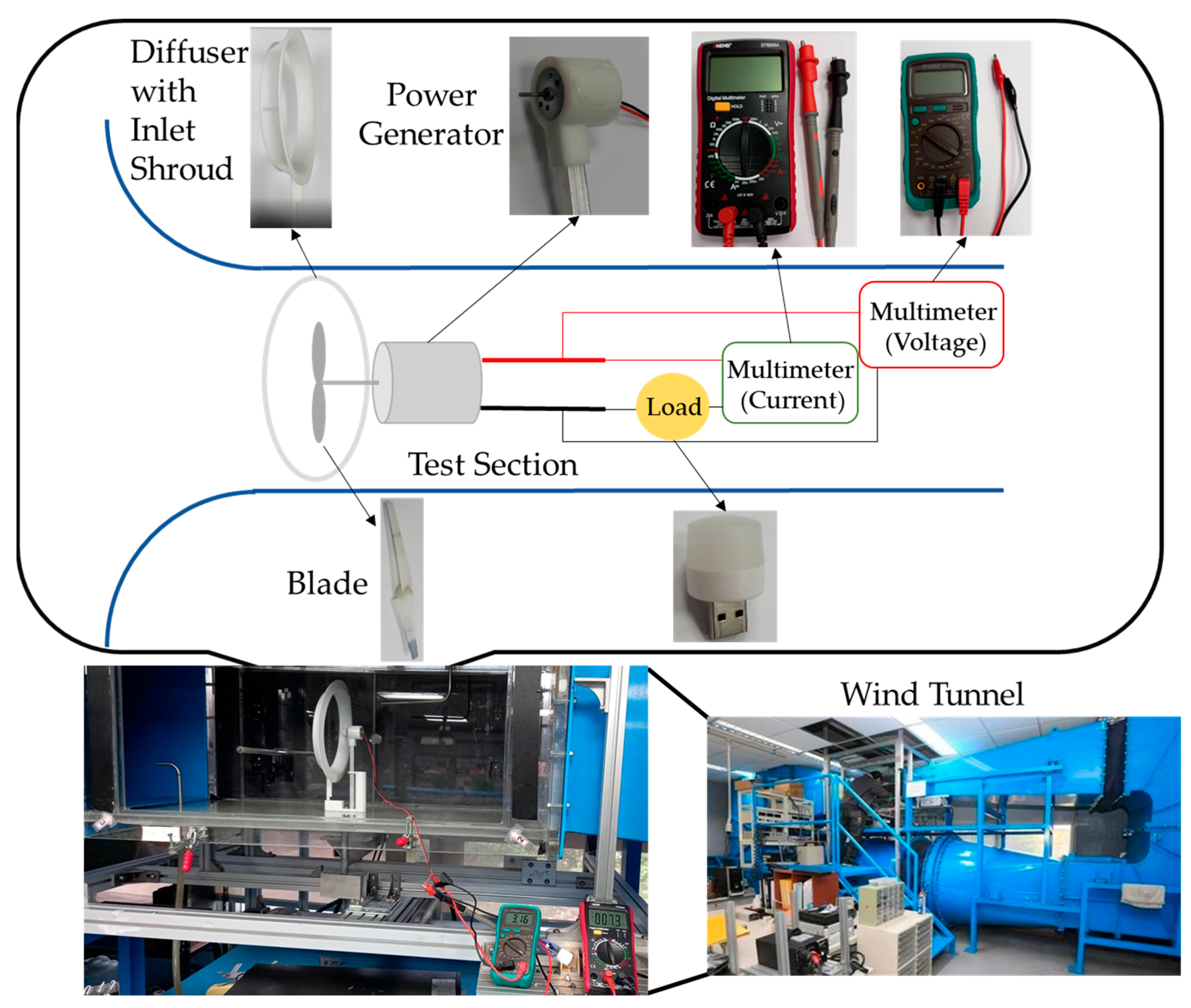
2.4. Experimental Setup and Measurement

In this study, 3D printing is used to establish a series of scaled-down basic and optimized DAWT models with a scale factor of 4/27 by considering the dimension of the wind tunnel test section, and wind tunnel experiments are conducted for effectiveness verification (Figure 5). The related equipment includes a power generator, electrical load, multimeters (current and voltage measurement), and the wind tunnel (including hot-wire speedometers, data acquisition systems, and experimental control software). For the experiments, the accuracies of the instruments used to measure the voltage and electric current are ±0.01 (brand/model: Pro’sKit/MT-1210) and ±0.025 (brand/model: ANENG/DT9205A), respectively. The following equations can be adopted to obtain the uncertainty of the measurement:
W = V I
δ W V = W V δ V = I δ V ,   δ W I = W I δ I = V δ I
u W , V = δ W V W = W V δ V W = V W W V δ V V = V W I δ V V = δ V V = u V
u W , I = δ W I W = W I δ I W = I W W V δ I I = I W V δ I I = δ I I = u I
u W = u W , V 2 + u W , I 2 1 / 2 = u V 2 + u I 2 1 / 2 = ± 0.01 2 + ± 0.025 2 = 2.7 %
where W is the power output, V is the voltage, I is the electric current, ui is the relative uncertainty of item i, and ui,j is the relative uncertainty of i in the result due to uncertainty in j. According to the above calculation, the uncertainty of the measured power output uW is 2.7%.

3. Results and Discussion

3.1. Numerical Validation

This study selects a two-blade design rotor proposed by Singh and Ahmed [72], which has lower construction costs and is suitable for low-wind speed applications. Its blade airfoil is an AF300, specially developed for low Re wind-turbine applications [78], as shown in Figure 6a. Figure 6 also displays the blade chord length and twist angle distributions of the rotor designed by Singh and Ahmed [72], which are used for constructing the blade solid model. The specifications of the rotor are presented in Table 1. The constructed rotor is placed in a size-verified computational domain (7D × 7D × 15D in x, y, and z directions, where D is the rotor diameter) with the origin located at the center of the rotor and its distance from the bottom ground is 4.5 m, as shown in Figure 7. The corresponding boundary conditions for the computational domain are also annotated in this figure. In addition, Figure 7 shows the receptor position for noise monitoring, where it is placed on the ground 5.635 m behind the wind turbine to comply with the international IEC 61400 standard [79], which specifies the angle between the line connecting the center of the wind turbine and the monitoring point along the ground is determined to be within 25° to 40°. A grid independence test proceeded, the predicted power variation was lower than 4%, and a grid number of about 9 × 10⁶ was employed for the following simulations. Figure 8 displays the mesh distribution around the rotor blade and the corresponding y+ values, whose maximum value is lower than 10. The predicted turbine power of the BWT with design rotational speed (ω = 500 rpm) under various wind speeds (U = 5–7 m/s) is compared with the experimental data presented by Sign and Ahmed [72], as shown in Figure 9. It can be found that the order of magnitude and trend of the predictions are generally consistent with the experimental data but are slightly overpredicted. The reason may be that the numerical simulation does not consider the energy conversion losses of the generator, so the predicted values are somewhat higher than the experimental values.
After validating the employed numerical procedure, diffusers will be introduced to enclose the rotor to form the DAWTs for subsequent evaluations under a wind velocity of U = 7 m/s. In this study, the diffuser profile of a cycloidal cure is used, following the recommendation of Ohya et al. [14]. The advantages of this implementation include the various inlet shrouds that will be introduced as the diffuser length changes, that various blade tip clearances will be introduced as the rotor axial position changes, and that various diffuser opening angles will also be introduced as the diffuser length and rotor axial position change. Adding an inlet shroud for the DAWT is recommended by researchers [29,35], who pointed out it can increase the approaching wind flow acceleration. Consideration of the tip clearance in the design of a DAWT is recommended by researchers [32,39], who point out that it is related to the aerodynamic and acoustic characteristics of the DAWTs. Diffuser opening angle was taken as a design parameter in studies performed by researchers [19,30,32,34], who revealed its significant effects on DAWT performance. In the summary of the papers surveyed, some key parameters regarding DAWT design have been collected, such as diffuser flange height/angle, diffuser profile/length/opening angle, rotor axial position, and blade tip clearance. The selected parameters adopted in this study are the diffuser’s flange height/angle, length, and rotor axial position, as indicated in Figure 1. After the cycloidal curve has been chosen as the diffuser profile, accompanied by the variations of selected parameters, the unselected parameters can also be included, and their effects can be involved. Table 2 shows the parameter ranges used in this study, specified according to the surveyed DAWT research works listed in Table 3. It can be found that the parameter ranges adopted all fall into the same order of magnitude as those used in other works. It is necessary to mention that the compact-type diffuser used by Ohya and Karasudani [14] was also utilized in this study to consider the structure’s strength.

3.2. Optimized Results Obtained by Taguchi Method

Since the Taguchi orthogonal array, a powerful statistical tool used in optimization processes [73], has been implemented to plan the design parameters to be utilized with the numerical simulations, the parameter ranges shown in Table 2 are divided into five levels for the DOE, as shown in Table 4. Thus, the Taguchi orthogonal array of L25(54) is yielded, creating 25 different geometric designs for the diffuser, so that the CFD simulations can be used to produce datasets for ML. At this step, a set of optimized parameters can also be gained using the Taguchi method for single-objective optimization. The Taguchi method uses a signal-to-noise (S/N) ratio, which renders a design quality and response graph to obtain the optimal parameters. Based on the 25 sets of generated power data from the CFD simulations, the corresponding S/N ratios can be calculated via Equation (14) for the cases of larger-the-better (LTB) characteristics.
S / N = 10 log M S D = 10 log 1 n i = 1 n 1 y i 2
where MSD is the mean square deviation indicating the average quality loss, n is the number of experiments, and yi is the i-th experiment quality characteristics. Figure 10 displays the response graph of the SN ratio for the LTB analysis of DAWT-generated power. Consequently, an optimized parameter combination can be obtained, as shown in Table 5, and labeled as DAWT-Taguchil, alongside an original design labeled as DAWT-Origina. The original one is set as level 1 of the studied parameters for reference. Figure 10 also indicates that the impact of the rotor’s axial position on the power output is the most significant, followed by the diffuser length, flange angle, and flange height.

3.3. Optimized Results Obtained by Multi-Objective Optimization

Before multi-objective optimization, besides the 25 datasets scheduled by the Taguchi orthogonal array, 45 randomly generated cases among the adopted parameter ranges (Table 2) are also used to conduct the CFD simulations prepared for BPNN training. The division between training and testing datasets was critical in effectively validating the BPNN model, and the detailed explanations are as follows:
  • Training dataset: The training set comprises a subset of the generated datasets obtained from the CFD simulations. This dataset trains the neural network model using the backpropagation algorithm. During training, the neural network learns the underlying patterns and the relationships between the input parameters (flange height/angle, diffuser length, rotor axial position) and the corresponding outputs (power output and generated noise of the DAWT). The Levenberg–Marquardt algorithm was employed in this phase to obtain a lower mean squared error [61].
  • Validation dataset: This dataset, separate from the training dataset, tunes hyperparameters and assesses the model’s performance during training. After each epoch of training iterations, the model’s performance is evaluated on the validation dataset to monitor the model’s generalization ability and prevent overfitting.
  • Test dataset: This dataset, separate from the training and validation datasets, is used to evaluate the final performance of the trained model and assess how well the trained model generalizes on unseen data.
Once the model is trained and tuned using the training and validation datasets, it is evaluated on the test dataset to estimate its performance in real-world scenarios. The results obtained from the test dataset provide an unbiased estimate of the model’s performance and help in making decisions about deploying the model in practical applications. In summary, the training dataset is used for model learning, the validation dataset is used for hyperparameter tuning and model evaluation during training, and the test dataset is used for final model evaluation to assess its performance on unseen data. Thus, the training dataset helps the model learn the proper patterns, the validation dataset helps developers fine-tune the model correctly, and the test dataset provides trustworthy metrics to deploy the predictions confidently.
The ratio of training, validation, and test datasets is 8:1:1. In our methodology, the activation functions used in the hidden and output layers of the neural network are hyperbolic tangent sigmoid and positive linear transfer functions, respectively. After evaluation, one hidden layer, eight neurons, and a learning rate 0.01 were adopted. Thus, we can accurately assess its ability to predict DAWT performance beyond the training data.
Based on the CFD results, Figure 11 displays the regression plot of the BPNN training, in which the input values are the design parameter conditions, the output values are the power and noise generated by DAWTs; it can be observed that the correlation coefficients R of the model training set, validating set, and testing set (the degree of fit of the data, the closer to 1, the better the degree of fit) are 0.99812, 0.99978, and 0.99915, respectively; all are greater than 0.99, which indicates that the overall estimation accuracy of the BPNN model is good.
This study employs the NSGA-II algorithm on the MATLAB platform, in which the GA operators include intermediate crossover, Gaussian mutation with a 100 initial population, 0.8 crossover rate, and a 300 maximum-number-of-generations adopted. Take the trained BPNN model as the fitness function of the NSGA-II algorithm for multi-objective optimization, and then the Pareto front can be obtained, as shown in Figure 12. There are Pareto-optimal solutions along the Pareto front, and different ones are chosen for various goals and labeled as NSGA-II-A, NSGA-II-B, and NSGA-II-C, among which NSGA-II-A focuses on power output, NSGA-II-C focuses on noise reduction, and NSGA-II-B focuses on both to achieve a compromise. Their corresponding parameter combinations are also listed in Table 5. Table 6 displays the comparison of power and noise values predicted by BPNN and CFD for the cases after the completion of the multi-objective optimization, while the other cases (DAWT-Original and DAWT-Taguchi) are included in the datasets primarily used for constructing the BPNN model, and thus their predicted values are not available. It can be found that the maximum error is almost less than 3%, except for the noise prediction of DAWT-NSGA-II-C, which is overpredicted but associated with the correct trend; the accuracy of the BPNN model is acceptable.
Table 7 shows the generated power and noise of various designs and their corresponding performance coefficients associated with the diffuser, i.e., backpressure, pressure recovery coefficients, and inflow velocity ratio, as proposed by Watanabe and Ohya [31]; their definitions are indicated in Equation (15).
C p b = p b p a 1 2 ρ U 2 ,   K = u 1 U ,   C p 2 = p 2 p a 1 2 ρ U 2 ,   C p d = C p   b   C p 2 K 2
where pa is the atmospheric pressure, pb is the back pressure behind the diffuser, p2 is the pressure behind the rotor, u1 is the wind speed in front of the rotor, and U is the upstream wind speed. Watanabe and Ohya [31] indicated that the back-pressure coefficient is significant for the performance of DAWTs and pointed out that a lower Cpb and a higher Cpd are desired for a high-performance DAWT. In addition, Table 7 displays the tip clearance for various designs, and it can be found that its original value of 10 mm will change with the selected parameter combinations during the optimization process, as mentioned before. Table 7 also displays these tip clearance values as divided by the rotor radius, which fall within a reasonable range, as presented in the literature [32,39].

3.4. Flow and Acoustic Fields: Analysis and Comparison

Table 7 shows that the generated power of the DAWTs is at least 37% higher than that of a BWT, which demonstrates the effectiveness of DAWT technology, and the sequence of magnitude, from high to low, is DAWT-NSGAII-A, DAWT-Taguchi, DAWT-NSGAII-B, DAWT-Original, DAWT-NSGAII-C, and BWT. In contrast, some of the noise levels generated by DAWTs are lower than that of a BWT, but some are greater, and the sequence of magnitude, from low to high, is DAWT-NSGAII-C, DAWT-Original, DAWT-NSGAII-B, BWT, DAWT-Taguchi, and DAWT-NSGAII-A. It should be noted that A-weighting [80], an effort to account for the relative loudness perceived by the human ear, is applied to measure the sound levels of noise in this study.
It can be found that DAWT-NSGAII-A, which focuses on power output, achieves the best power output values with the highest noise level. Meanwhile, DAWT-NSGAII-B considers both output power and noise reduction; although it is slightly lower in power output than DAWT-Taguchi, it exhibits better noise-reduction performance. Moreover, its noise level is lower than that of BWT, unlike DAWT-Taguchi, which exceeds that of BWT. As for DAWT-Taguchi, its performance is quite reasonable, considering that its optimization is aimed at power output. After all, its configuration is optimized for power output, so its noise-reduction performance can be expected. As for DAWT-NSGAII-C, which emphasizes noise reduction, although its power output is the lowest, it still exceeds that of the BWT, and its noise reduction performance is quite good. The above results demonstrate the considerable success of ML optimization. Using the optimization results mentioned above, this study will analyze the flow and acoustic fields to understand their relevant characteristics better.
The comparison of pressure distributions (Figure 13) shows that the bare wind turbine exhibits fewer pronounced pressure gradients than the wind turbine with a diffuser. Consequently, it cannot form an adequate pressure difference around the rotor to drive the flow field to increase the airflow speed. Conversely, the diffuser’s placement can generate more distinct pressure gradients around the rotor, thus augmenting airflow velocity, and assisting the rotor’s work. Such phenomena are consistent with their power output values. Notably, the diffuser designed by ML (DAWT-NSGAII-A) creates the most pronounced pressure gradient (Figure 13d), as expected.
The inflow velocity ratio (K) indicated in Table 7 displays a magnitude sequence of DAWT-NSGAII-B, DAWT-NSGAII-A, DAWT-Taguchi, DAWT-NSGAII-C, DAWT-Original, and BWT, which is not consistent with their sequence as to power output, i.e., DAWT-NSGAII-A, DAWT-Taguchi, DAWT-NSGAII-B, DAWT-Original, DAWT-NSGAII-C, and BWT. The reason why DAWT-NSGAII-B exhibits the highest K but produces less output power than DAWT-NSGAII-A and DAWT-Taguchi can be determined by observing the axial pressure and velocity distributions shown in Figure 13 and Figure 14. Because its rotor axial position is the closest to the diffuser exit (Table 5), the high-velocity region behind the diffuser exit is closer to the rotor (Figure 14e) and this makes it exhibit the highest K, and so demonstrate the lowest Cpb (Table 7). However, such a geometric arrangement causes it to have the poorest Cpd and exhibit a weaker pressure gradient near the rotor (Figure 13e). Such flow characteristics are helpful to noise reduction and enable DAWT-NSGAII-B to balance both design objectives. Similar phenomena, e.g., higher K does not produce higher power output, can be observed with the DAWT-Original and DAWT-NSGAII-C, but another reason causes this. The rotor axial positions of both designs are not too different (1 and 1.4, as indicated in Table 5). Because K is an area-averaged value, it cannot reflect the different space distributions of the flow field. By observing Figure 14b,f, it can be determined that the high-velocity regions of both DAWT-Original and DAWT-NSGA-II-C are closer to the diffuser peripheral and farther from the rotor. Based on the observation of pressure and velocity fields, it can be concluded that adding a diffuser enhances the mass flow rate of the airflow that passes through the rotor, and increases its power output.
Figure 15 shows the Y-component vorticity and velocity vector distributions. By comparing the strengths of the vorticity, it is easy to determine that DAWT-NSGAII-A and DAWT-Taguchi both exhibit stronger vortices, producing higher power output. Both designs implement higher flange heights and rotor axial positions closer to the diffuser exit, resulting in the flow structures shown in Figure 15. Such a design can augment the power output but increase the noise intensity due to the strong vortices produced.
Figure 16 and Figure 17 show the original noise spectrum and the one processed with A-weighting. In terms of noise, the frequency range audible to the human ear is from 20 Hz to 20 kHz. Observing these figures shows that adding a diffuser can suppress the noise in the frequency band of 200 Hz to 800 Hz. But suppose the added diffuser produces strong vortices in the flow field. In that case, the noise in the lower frequency band of 80 Hz to 200 Hz will be raised, resulting in a negative effect on noise reduction, i.e., not suppressing the noise, but intensifying it. This observation might explain why inconsistency assessment exists in the literature [11,25,38,51] discussing the addition of a diffuser that may suppress or intensify the noise.
Figure 18 shows the isosurface of acoustic power with 20 dB and acoustic power contour on the Y-Z plane (X/D = 0). This physical quantity is calculated by Equation (6) and is related to turbulent shear stress in the flow. It can be found that the most vital region of acoustic power for the DAWT is near the space between the blade tip and the diffuser’s inner wall, as shown in Figure 18. By comparing Figure 15c–e, Figure 16c–e and Figure 17c–e, it is evident that the tip vortices generated in those DAWTs induce more substantial turbulence, causing locally higher turbulent shear stress, which intensifies the noise in a lower frequency band. This interpretation can be further verified by observing the turbulent kinetic energy (TKE) distribution displayed in Figure 19 (the intensity of TKE isosurface is 4 m2/s2), which has almost the same form as the acoustic power distribution. Figure 20 displays the acoustic surface power, calculated by Equation (7), which is related to the pressure fluctuations in the flow field. Observing this figure shows that the intensity of acoustic surface power on the blade surface is almost the same for all cases, including the BWT. It can be inferred that the primary noise source is the pressure fluctuation produced by the rotating blade, and the imposition of a diffuser will mitigate its contribution to the overall noise in the frequency band of 200 Hz to 800 Hz.
By further observing Table 5, it can be determined that the case with the highest diffuser flange height is DAWT-NSGA-II-A, which is optimized for focusing on the power output, while the lowest one is DAWT-Original, the case of the original design. This observation implies that the higher the flange height, the more power output may be obtained if the effects of the other parameters and structural strength problems are not considered. According to the pressure, velocity, and vorticity fields displayed (Figure 13, Figure 14 and Figure 15), a higher diffuser flange height will induce a larger recirculation zone with lower pressure and stronger vorticity, shifting the recirculation zone away from the rotor. It also can be noted that the higher flange height makes the noise spectrum around the frequency band of 80–800 Hz more intense, especially 200–800 Hz (Figure 17), accompanied by more acoustic power (Figure 18) and acoustic surface power (Figure 20), which are caused by the strongly induced vortices and fluctuating pressure among the region of the blade tip and the flange’s rear part.
Table 5 also shows that the only one with a negative flange angle is DAWT-NSGA-II-B, which makes the air flow more smoothly through the device. Interestingly, compounded with other parameters, the negative flange angle can compromise power output and noise generation. In such a way, it exhibits a relatively good back-pressure coefficient but a poor pressure recovery coefficient (Table 7). It helps accelerate the flow, with a more substantial pressure difference with strong induced vortices but with less slow pressure recovery as it flows downstream. This phenomenon is evident in its intensified noise spectrum around the frequency band of 80–200 Hz, as shown in Figure 17e, originating from medium-strong vortices, and less acoustic surface power means fewer pressure fluctuations, as shown in Figure 20e.
It is worth mentioning that with the cycloidal diffuser profile adopted, as both parameters change, i.e., diffuser length and rotor axial position, the effects of tip clearance, adding of inlet shroud, and diffuser opening angle are involved implicitly. In such a situation, the studied design parameters interact intricately, making conducting systematic analyses using conventional parametric studies hard. The proposed methodology provides a feasible approach to overcome this difficulty.
Figure 21 displays the power coefficients (Cp) of the DAWTs analyzed in this study and compares them with the ones of typical BWTs presented in Ref. [8]. The definition of Cp is shown in Equation (16).
C p = P 1 2 ρ U 3 A d
where P is the power output of DAWT, and Ad is the cross-section area of the diffuser. It can be found that the optimized designs proposed in this study provide reasonable power performance. By inspecting the definition presented in Equation (16), it can be recognized that DAWTs implemented with high flange height will decrease their Cp value if their output power increases cannot compensate for the increased area. Figure 22 shows the experimental measurement results of the scaled-down DAWT models manufactured by 3D printing. It can be found that the sequence of the magnitudes of measured output power almost displays the same trend as the full-scale CFD simulations of the optimized designs. Thus, this can verify the effectiveness of the optimization methodology proposed in this study even though all the results presented in this paper are achieved without considering the manufacturing costs, structural strength, energy conversion efficiency of the electric generator, friction loss of the gearbox, and bearing power loss. In addition, both the BPNN and NSGA-II algorithms are potent tools for predictive and optimization modeling. However, they also have certain limitations; e.g., BPNN may suffer from issues about local minima, overfitting, gradient vanishing/exploding, hyperparameter sensitivity, etc.; NSGA-II may encounter problems with convergence, premature convergence, scalability, parameter sensitivity, etc. In summary, while both BPNN and NSGA-II offer valuable capabilities for optimization and modeling tasks, researchers and practitioners should be mindful of their limitations and employ them with careful and deliberate testing and evaluation, using the latest-version models and suitable platforms, to address specific challenges effectively.

4. Conclusions

This study synergistically implements validated CFD and ML techniques to optimize a two-blade DAWT suitable for low-wind speed area applications. The research parameters include the diffuser’s flange height/angle, the diffuser’s length, and the rotor’s axial position. The primary conclusions of this study are as follows:
1.
This study successfully integrates CFD, BPNN, and NSGA-II to conduct multi-objective optimization of DAWT, using output power and noise as objective functions. Performance evaluation and verification are carried out for the optimized designs. Finally, the diffuser configurations that meet different requirements for power and noise are proposed.
2.
The influence of design parameters can be evaluated through the Taguchi method. It was found that the impact of the rotor’s axial position on the power output of DAWT is the most significant, followed by those of the diffuser length, flange angle, and height.
3.
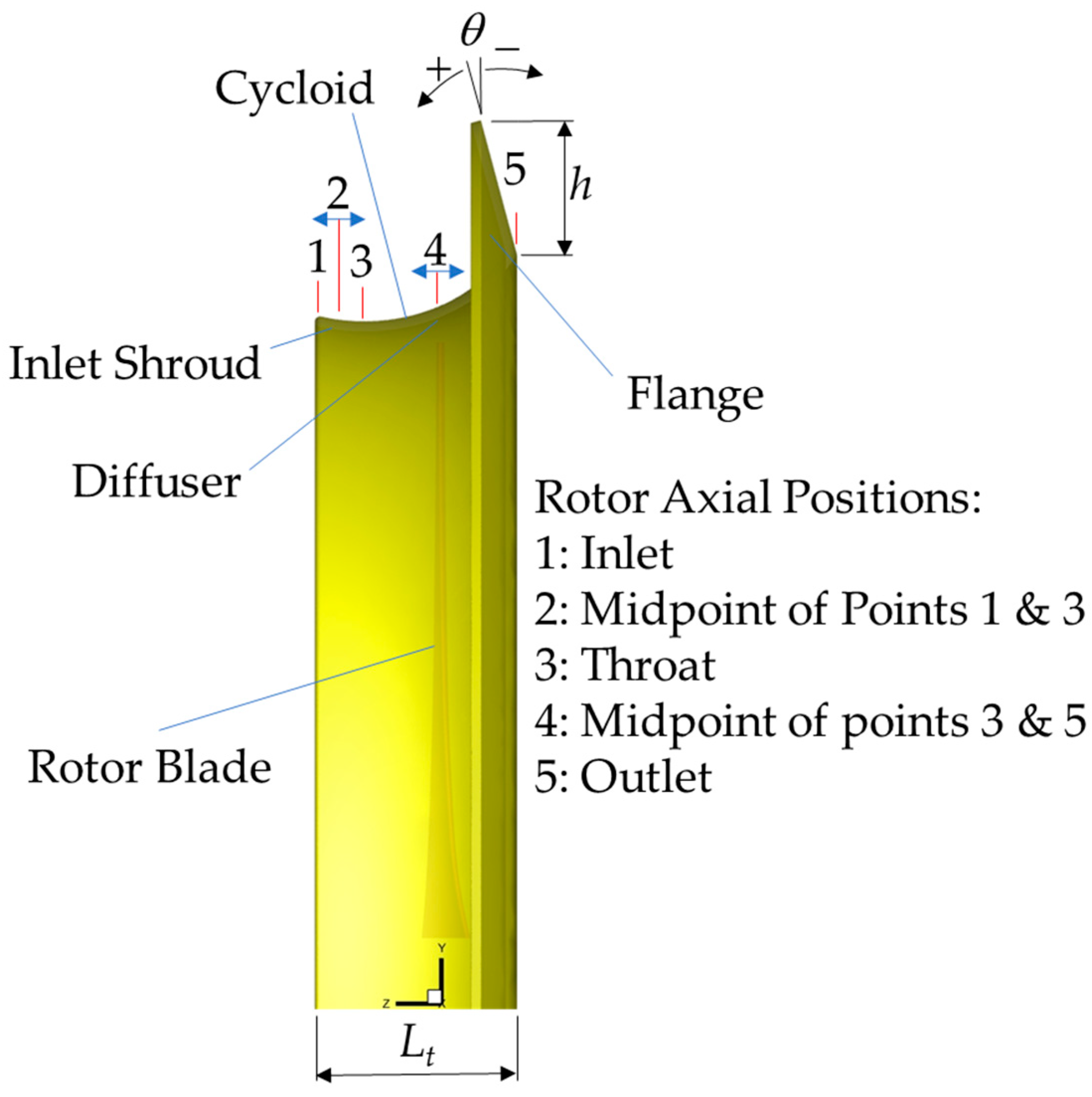
When employing a cycloid diffuser profile, varying the design parameters, i.e., flange height/angle, diffuser length, and rotor axial position, allows for the indirect incorporation of additional parameters, i.e., tip clearance, diffuser opening angle, and the adding of inlet shroud, allowing these values to be optimized together.
4.
It was evident that a well-designed diffuser requires the acceleration of airflow while maintaining high-pressure recovery.
5.
Under the conditions of this study, introducing a diffuser can reduce the noise in the frequency band of 200 Hz to 800 Hz, but if the induced tip vortex is too strong, it will have the opposite effect on the noise reduction. This finding can be used to interpret the positive and negative impacts on noise of installing a diffuser.
6.
The flange height should not be too high or too low. If it is too low, it will not be able to generate a vortex with sufficient strength behind it to accelerate the airflow inside the diffuser, which will provide limited help to the power output. However, if the flange is too high, it will cause the recirculation zone to be far away from the rotor inside the diffuser, resulting in limited benefit to power output. Moreover, if the flange height is too high, it would lead to structural damage and deformation, resulting in higher maintenance costs and making it unsuitable for practical applications.
7.
An appropriate flange angle can induce vortices to drive and accelerate airflow within the diffuser. Negative flange angles balance power and noise demands, resulting in smoother flow fields with weaker pressure fluctuations and lower noise levels.
8.
If the diffuser length is too long, it is unsuitable for practical applications because it can cause the DAWT to be too heavy for placement in elevated locations. Additionally, excessive length can hinder the vortices generated by the flange from influencing the flow field near the rotor inside the diffuser.
9.
The rotor should ideally be positioned behind the throat (approximately halfway between the throat and the outlet) to receive the accelerated flow field induced by the vortices generated by the flange, thereby enhancing its power output. Placing the rotor near this position between the throat and the outlet yields better results for maximizing power output. However, positioning the rotor in front of the throat is more effective for noise reduction.

Author Contributions

Conceptualization, P.-W.H., J.-H.W. and Y.-J.C.; methodology, P.-W.H.; software, J.-H.W.; validation, P.-W.H. and J.-H.W.; formal analysis, P.-W.H. and J.-H.W.; investigation, P.-W.H. and J.-H.W.; resources, P.-W.H. and Y.-J.C.; data curation, P.-W.H. and J.-H.W.; writing—original draft preparation, P.-W.H. and J.-H.W.; writing—review and editing, P.-W.H.; visualization, P.-W.H.; supervision, P.-W.H.; project administration, P.-W.H.; funding acquisition, P.-W.H. and Y.-J.C. All authors have read and agreed to the published version of the manuscript.

Funding

We would like to thank The National Science and Technology Council, Taiwan, for financing the development of this research, with project number 110-2221-E-035-051.

Institutional Review Board Statement

Not applicable.

Informed Consent Statement

Not applicable.

Data Availability Statement

The data presented in this study are included in the article; further inquiries can be directed to the corresponding author.

Conflicts of Interest

The authors declare no conflicts of interest.

References

  1. Gayen, D.; Chatterjee, R.; Roy, S. A review on environmental impacts of renewable energy for sustainable development. Int. J. Environ. Sci. Technol. 2024, 21, 5285–5310. [Google Scholar] [CrossRef]
  2. Sayed, E.T.; Wilberforce, T.; Elsaid, K.; Rabaia, M.K.H.; Abdelkareem, M.A.; Chae, K.J.; Olabi, A.G. A critical review on environmental impacts of renewable energy systems and mitigation strategies: Wind, hydro, biomass and geothermal. Sci. Total Environ. 2021, 766, 144505. [Google Scholar] [CrossRef] [PubMed]
  3. Darwish, A.S.; Al-Dabbagh, R. Wind energy state of the art: Present and future technology advancements. Renew. Energy Environ. Sustain. 2020, 5, 7. [Google Scholar] [CrossRef]
  4. Nazir, M.S.; Ali, N.; Bilal, M.; Iqbal, H.M.N. Potential environmental impacts of wind energy development: A global perspective. Curr. Opin. Environ. Sci. Health 2020, 13, 85–90. [Google Scholar] [CrossRef]
  5. Joselin Herbert, G.M.; Iniyan, S.; Sreevalsanc, E.; Rajapandian, S. A review on wind energy technologies. Renew. Sustain. Energy Rev. 2007, 11, 1117–1145. [Google Scholar] [CrossRef]
  6. Hutchinson, M.; Zhao, F. GWEC|Global Wind Report 2023; Global Wind Energy Council: Brussels, Belgium, 2023. [Google Scholar]
  7. Kassa, B.Y.; Baheta, A.T.; Beyene, A. Current trends and innovations in enhancing the aerodynamic performance of small-scale, horizontal axis wind turbines: A review. ASME Open J. Eng. 2024, 3, 031001. [Google Scholar] [CrossRef]
  8. Burton, T.; Jenkins, N.; Bossanyi, E.; Sharpe, D.; Graham, M. Wind Energy Handbook, 3rd ed.; John Wiley & Sons, Ltd.: West Sussex, UK, 2021. [Google Scholar]
  9. Alabdali, Q.A.; Bajawi, A.M.; Fatani, A.M.; Nahhas, A.M. Review of recent advances of wind energy. Sustain. Energy 2020, 8, 12–19. [Google Scholar]
  10. Jianu, O.; Rosen, M.A.; Naterer, G. Noise pollution prevention in wind turbines: Status and recent advances. Sustainability 2012, 4, 1104–1117. [Google Scholar] [CrossRef]
  11. Ohya, Y.; Karasudani, T.; Nagai, T.; Watanabe, K. Wind lens technology and its application to wind and water turbine and beyond. Renew. Energy Environ. Sustain. 2017, 2, 2. [Google Scholar] [CrossRef]
  12. Nunes, M.M.; Brasil Junior, A.C.P.; Oliveira, T.F. Systematic review of diffuser-augmented horizontal-axis turbines. Renew. Sustain. Energy Rev. 2020, 133, 110075. [Google Scholar] [CrossRef]
  13. Ilhan, A.; Sahin, B.; Bilgili, M. A review: Diffuser augmented wind turbine technologies. Int. J. Green Energy 2022, 19, 1–27. [Google Scholar] [CrossRef]
  14. Ohya, Y.; Karasudani, T. A shrouded wind turbine generating high output power with wind-lens technology. Energies 2010, 3, 634–649. [Google Scholar] [CrossRef]
  15. Watson, S.; Moro, A.; Reis, V.; Baniotopoulos, C.; Barth, S.; Bartoli, G.; Bauer, F.; Boelman, E.; Bosse, D.; Cherubini, A.; et al. Future emerging technologies in the wind power sector: A European perspective. Renew. Sustain. Energy Rev. 2019, 113, 109270. [Google Scholar] [CrossRef]
  16. Calautit, K.; Johnstone, C. State-of-the-art review of micro to small-scale wind energy harvesting technologies for building integration. Energy Convers. Manag. X 2023, 20, 100457. [Google Scholar] [CrossRef]
  17. Al-Quraishi, B.A.J.; Asmuin, N.Z.B.; Mohd, S.B.; Abd Al-Wahid, W.A.; Mohammed, A.N.; Didane, D.H. Review on diffuser augmented wind turbine (DAWT). Int. J. Integr. Eng. 2019, 11, 178–206. [Google Scholar] [CrossRef]
  18. Aravindhan, N.; Bibin, C.; Kumar, R.A.; Kalyan, K.S.; Balaji, K.S.; Kugan, R.; Rajesh, K.; Arunkumar, S. Performance analysis of various types of ducted wind turbines—A review. Mater. Today Proc. 2023, 80, 188–194. [Google Scholar] [CrossRef]
  19. Abe, K.I.; Ohya, Y. An investigation of flow fields around flanged diffusers using CFD. J. Wind. Eng. Ind. Aerodyn. 2004, 92, 315–330. [Google Scholar] [CrossRef]
  20. Abe, K.; Nishida, M.; Sakurai, A.; Ohya, Y.; Kihara, H.; Wada, E.; Sato, K. Experimental and numerical investigations of flow fields behind a small wind turbine with a flanged diffuser. J. Wind. Eng. Ind. Aerodyn. 2005, 93, 951–970. [Google Scholar] [CrossRef]
  21. Toshimitsu, K.; Nishikawa, K.; Haruki, W.; Oono, S.; Takao, M.; Ohya, Y. PIV measurements of flows around the wind turbines with a flanged-diffuser shroud. J. Therm. Sci. 2008, 17, 375–380. [Google Scholar] [CrossRef]
  22. Jafari, S.A.H.; Kosasih, B. Flow analysis of shrouded small wind turbine with a simple frustum diffuser with computational fluid dynamics simulations. J. Wind Eng. 2014, 125, 102–110. [Google Scholar] [CrossRef]
  23. Roshan, S.Z.; Alimirzazadeh, S.; Rad, M. RANS simulations of the stepped duct effect on the performance of ducted wind turbine. J. Wind. Eng. Ind. Aerodyn. 2015, 145, 270–279. [Google Scholar] [CrossRef]
  24. El-Zahaby, A.M.; Kabeel, A.E.; Elsayed, S.S.; Obiaa, M.F. CFD analysis of flow fields for shrouded wind turbine’s diffuser model with different flange angles. Alex. Eng. J. 2017, 56, 171–179. [Google Scholar] [CrossRef]
  25. Amano, R.S. Review of wind turbine research in 21st Century. J. Energy Resour. Technol. 2017, 139, 050801. [Google Scholar] [CrossRef]
  26. Natesan, M.; Jeyanthi, S.; Sivasathya, U. A review on design of augmented wind turbine blade for low wind speed urban area. Int. J. Mech. Eng. Technol. 2017, 8, 685–691. [Google Scholar]
  27. Heikal, H.A.; Abu-Elyazeed, O.S.M.; Nawar, M.A.A.; Attai, Y.A. On the actual power coefficient by theoretical developing of the diffuser flange of wind-lens turbine. Renew. Energy 2018, 125, 295–305. [Google Scholar] [CrossRef]
  28. Klistafani, Y.; Mukhsen, M.I. Development of a shrouded wind turbine with various diffuser type structures. IOP Conf. Ser. Mater. Sci. Eng. 2019, 676, 012040. [Google Scholar] [CrossRef]
  29. Anbarsooz, M.; Mazloum, M.; Moghadam, D.G. Converging-diverging ducts for efficient utilization of low-grade wind energy: Numerical and experimental studies. J. Renew. Sustain. Energy 2020, 12, 023304. [Google Scholar] [CrossRef]
  30. Arifin, F.; Kusumanto, R.D.; Bow, Y.; Rusdianasari; Taqwa, A.; Susandi, A.; Herlambang, Y.D.; Wang, M.W.; Sitompul, C.R. Study the effect diffuser length and degree to horizontal wind turbine. In Proceedings of the 4th International Conference on Applied Science and Technology on Engineering Science (iCAST-ES 2021), Samarinda, Indonesia, 23–24 October 2021. [Google Scholar]
  31. Watanabe, K.; Ohya, Y. A Simple theory and performance prediction for a shrouded wind turbine with a brimmed diffuser. Energies 2021, 14, 3661. [Google Scholar] [CrossRef]
  32. Ramayee, L.; Supradeepan, K. Influence of axial distance and duct angle in the improvement of power generation in duct augmented wind turbines. J. Energy Resour. Technol. Trans. ASME 2022, 144, 091302. [Google Scholar] [CrossRef]
  33. Hashem, I.; Hafiz, A.A.; Mohamed, M.H. Characterization of aerodynamic performance of wind-lens turbine using high-fidelity CFD simulations. Front. Energy 2022, 16, 661–682. [Google Scholar] [CrossRef]
  34. Jauhar, T.A.; Hussain, M.I.; Kiren, T.; Arif, W.; Miran, S.; Lee, G.H. Effect of flanged diffuser divergence angle on wind turbine: A numerical investigation. PLoS ONE 2023, 18, e0287053. [Google Scholar] [CrossRef]
  35. Mutasher, S.A.; Ahmed, H.M. CFD analysis of brimmed diffuser augmented wind turbine. In Proceedings of the 2023 IEEE 8th International Conference on Engineering Technologies and Applied Sciences (ICETAS), InterContinental Bahrain, Manama, Bahrain, 25–27 October 2023. [Google Scholar]
  36. Göçmen, T.; Özerdema, B. Airfoil optimization for noise emission problem and aerodynamic performance criterion on small scale wind turbines. Energy 2012, 46, 62–71. [Google Scholar] [CrossRef]
  37. Reja, R.K.; Amin, R.; Tasneem, Z.; Ali, M.F.; Islam, M.R.; Saha, D.K.; Badal, F.R.; Ahamed, M.H.; Moyeen, S.I.; Das, S.K. A review of the evaluation of urban wind resources: Challenges and perspectives. Energy Build. 2022, 257, 111781. [Google Scholar] [CrossRef]
  38. Hashem, I.; Mohamed, M.H.; Hafiz, A.A. Aero-acoustics noise assessment for wind-lens turbine. Energy 2017, 118, 345–368. [Google Scholar] [CrossRef]
  39. Avallone, F.; Ragni, D.; Casalino, D. On the effect of the tip-clearance ratio on the aeroacoustics of a diffuser-augmented wind turbine. Renew. Energy 2020, 152, 1317–1327. [Google Scholar] [CrossRef]
  40. Sanderse, B.; van der Pijl, S.P.; Koren, B. Review of computational fluid dynamics for wind-turbine wake aerodynamics. Wind Energy 2011, 14, 797–819. [Google Scholar] [CrossRef]
  41. Rehman, S.; Alam, M.M.; Alhems, L.M.; Rafique, M.M. Horizontal axis wind turbine blade design methodologies for efficiency enhancement—A review. Energies 2018, 11, 506. [Google Scholar] [CrossRef]
  42. Agha, A.; Chaudhry, H.N.; Wang, F. Diffuser augmented wind turbine (DAWT) technologies: A review. Int. J. Renew. Energy Res. 2018, 8, 1369–1385. [Google Scholar]
  43. Marugán, A.P.; Márquez, F.P.G.; Perez, J.M.P.; Ruiz-Hernández, D. A survey of artificial neural network in wind energy systems. Appl. Energy 2018, 228, 1822–1836. [Google Scholar] [CrossRef]
  44. Elyasichamazkoti, F.; Khajehpoor, A. Application of machine learning for wind energy from design to energy-Water nexus: A Survey. Energy Nexus 2021, 2, 100011. [Google Scholar] [CrossRef]
  45. Bin Abu Sofian, A.D.A.; Lim, H.R.; Siti Halimatul Munawaroh, H.; Ma, Z.; Chew, K.W.; Show, P.L. Machine learning and the renewable energy revolution: Exploring solar and wind energy solutions for a sustainable future including innovations in energy storage. Sustain. Dev. 2024, 1–26. [Google Scholar] [CrossRef]
  46. Nikolić, V.; Petković, D.; Shamshirband, S.; Ćojbašić, Ž. Adaptive neuro-fuzzy estimation of diffuser effects on wind turbine performance. Energy 2015, 89, 324–333. [Google Scholar] [CrossRef]
  47. Liu, J.; Song, M.; Chen, K.; Wu, B.; Zhang, X. An optimization methodology for wind lens profile using computational fluid dynamics simulation. Energy 2016, 109, 602–611. [Google Scholar] [CrossRef]
  48. Oka, N.; Furukawa, M.; Kawamitsu, K.; Yamada, K. Optimum aerodynamic design for wind-lens turbine. J. Fluid Sci. Technol. 2016, 11, JFST0011. [Google Scholar] [CrossRef]
  49. Khamlaj, T.A.; Rumpfkeil, M.P. Analysis and optimization of ducted wind turbines. Energy 2018, 162, 1234–1252. [Google Scholar] [CrossRef]
  50. Leloudas, S.N.; Lygidakis, G.N.; Eskantar, A.I.; Nikolos, I.K. A robust methodology for the design optimization of diffuser augmented wind turbine shrouds. Renew. Energy 2020, 150, 722–742. [Google Scholar] [CrossRef]
  51. Rahmatian, M.A.; Shahrbabaki, A.N.; Moeini, S.P. Single-objective optimization design of convergent-divergent ducts of ducted wind turbine using RSM and GA, to increase power coefficient of a small-scale horizontal axis wind turbine. Energy 2023, 269, 126822. [Google Scholar] [CrossRef]
  52. Shambira, N.; Makaka, G.; Mukumba, P. Velocity augmentation model for an empty concentrator-diffuser-augmented wind turbine and optimisation of geometrical parameters using surface response methodology. Sustainability 2024, 16, 1707. [Google Scholar] [CrossRef]
  53. Kuninti, S.; Rooban, S. Backpropagation algorithm and its hardware implementations: A review. J. Phys. Conf. Ser. 2021, 1804, 012169. [Google Scholar] [CrossRef]
  54. Solanki, S.; Jethva, H.B. A review on back propagation algorithms for feedforward networks. Glob. Res. Anal. 2013, 2, 73–75. [Google Scholar] [CrossRef]
  55. Rumelhart, D.E.; Hinton, G.E.; Williams, R.J. Learning internal representations by error propagation. In Parallel Distributed Processing: Explorations in the Microstructure of Cognition; Rumelhart, D.E., McClelland, J.L., Eds.; The MIT Press: Cambridge, MA, USA, 1986; Volume 1, pp. 318–362. [Google Scholar]
  56. Li, M. Comprehensive review of backpropagation neural networks. Acad. J. Sci. Technol. 2024, 9, 150–154. [Google Scholar] [CrossRef]
  57. Lillicrap, T.P.; Santoro, A.; Marris, L.; Akerman, C.J.; Hinton, C. Backpropagation and the brain. Nat. Rev. Neurosci. 2020, 21, 335–346. [Google Scholar] [CrossRef]
  58. Suliman, A.; Zhang, Y. A review on back-propagation neural networks in the application of remote sensing image classification. J. Earth Sci. Eng. 2015, 5, 52–65. [Google Scholar]
  59. Primadusi, U.; Cahyadi, A.I.; Prasetyo, D.; Wahyunggoro, O. Backpropagation neural network models for LiFePO4 Battery. AIP Conf. Proc. 2016, 1755, 090009. [Google Scholar]
  60. Jwo, D.J.; Biswal, A.; Mir, I.A. Artificial neural networks for navigation systems: A review of recent research. Appl. Sci. 2023, 13, 4475. [Google Scholar] [CrossRef]
  61. Nguyen, T.A.; Ly, H.B.; Pham, B.T. Backpropagation neural network-based machine learning model for prediction of soil friction angle. Math. Probl. Eng. 2020, 2020, 8845768. [Google Scholar] [CrossRef]
  62. Coley, D.A. An Introduction to Genetic Algorithms for Scientists and Engineers, 1st ed.; World Scientific Publishing Company: Danvers, MA, USA, 1999; pp. 2–3. [Google Scholar]
  63. Cerf, S.; Doerr, B.; Hebras, B.; Kahane, Y.; Wietheger, S. The first proven performance guarantees for the non-dominated sorting genetic algorithm II (NSGA-II) on a combinatorial optimization problem. In Proceedings of the 32nd International Joint Conference on Artificial Intelligence, Macao SAR, China, 19–25 August 2023. [Google Scholar]
  64. Qu, Y.; Ma, Z.; Clausen, A.; Jørgensen, B.N. A comprehensive review on evolutionary algorithm solving multi-objective Problems. In Proceedings of the 22nd IEEE International Conference on Industrial Technology (ICIT), Valencia, Spain, 10–12 March 2021. [Google Scholar]
  65. Deb, K.; Pratap, A.; Agarwal, S.; Meyarivan, T. A fast and elitist multi-objective genetic algorithm: NSGA-II. IEEE Trans. Evol. Comput. 2002, 6, 182–197. [Google Scholar] [CrossRef]
  66. Damak, N.; Jarboui, B.; Loukil, T. Non-dominated sorting genetic algorithm-II to solve bi-objective multi-mode resource-constrained project scheduling. In Proceedings of the 2013 International Conference on Control, Decision and Information Technologies (CoDIT), Hammamet, Tunisia, 6–8 May 2013. [Google Scholar]
  67. Verma, S.; Pant, M.; Snasel, V. A comprehensive review on NSGA-II for multi-objective combinatorial optimization problems. IEEE Access 2021, 9, 57757–57791. [Google Scholar] [CrossRef]
  68. Golchha, A.; Qureshi, S.G. Non-dominated sorting genetic algorithm-II—A succinct survey. Int. J. Comput. Sci. Inf. Technol. 2015, 6, 252–255. [Google Scholar]
  69. Rahimi, I.; Gandomi, A.H.; Deb, K.; Chen, F.; Nikoo, M.R. Scheduling by NSGA-II: Review and bibliometric analysis. Processes 2022, 10, 98. [Google Scholar] [CrossRef]
  70. Ma, H.; Zhang, Y.; Sun, S.; Liu, T.; Shan, Y. A comprehensive survey on NSGA-II for multi-objective optimization and applications. Artif. Intell. Rev. 2023, 56, 15217–15270. [Google Scholar] [CrossRef]
  71. Chang, H.; Zhang, G.; Sun, Y.; Lu, S. Non-dominant genetic algorithm for multi-objective optimization design of unmanned aerial vehicle shell process. Polymers 2022, 14, 2896. [Google Scholar] [CrossRef]
  72. Singh, R.K.; Ahmed, M.R. Blade design and performance testing of a small wind turbine rotor for low wind speed applications. Renew. Energy 2013, 50, 812–819. [Google Scholar] [CrossRef]
  73. Taguchi, G. System of Experimental Design: Engineering Methods to Optimize Quality and Minimize Costs, 1st ed.; UNIPUB/Kraus International Publications: Dearborn, MI, USA, 1987; pp. 653–655. [Google Scholar]
  74. Menter, F.R. Two-equation eddy-viscosity turbulence models for engineering applications. AIAA J. 1994, 32, 1598–1605. [Google Scholar] [CrossRef]
  75. Ffowcs-Williams, J.E.; Hawkings, D.L. Sound generation by turbulence and surfaces in arbitrary motion. Proc. R. Soc. A Math. Phys. Eng. Sci. 1969, 264, 321–342. [Google Scholar]
  76. Proudman, I. The generation of noise by isotropic turbulence. Proc. R. Soc. A Math. Phys. Eng. Sci. 1952, 214, 119–132. [Google Scholar]
  77. Curle, N. The influence of solid boundaries upon aerodynamic sound. Proc. R. Soc. A Math. Phys. Eng. Sci. 1955, 231, 505–514. [Google Scholar]
  78. Singh, R.K.; Ahmed, M.R.; Zullah, M.A.; Lee, Y.H. Design of a low Reynolds number airfoil for small horizontal axis wind turbines. Renew. Energy 2012, 42, 66–76. [Google Scholar] [CrossRef]
  79. IEC 61400-11; International Standard, Wind Turbines–Part 11: Acoustic Noise Measurement Techniques. International Electrotechnical Commission: Geneva, Switzerland, 2018.
  80. IEC 61672-1:2013; Electroacoustics–Sound Level Meters–Part 1: Specifications. International Electrotechnical Commission: Geneva, Switzerland, 2013.
Figure 1. Illustration of the principal components and geometric parameters of the studied diffuser-augmented wind turbine with inlet shroud.
Sustainability 16 03648 g001
Figure 2. Flowchart with a schematic diagram of the research.
Sustainability 16 03648 g002
Figure 3. The architecture of the backpropagation neural network (BPNN).
Sustainability 16 03648 g003
Figure 4. Flowchart of the NSGA-II algorithm.
Sustainability 16 03648 g004
Figure 5. Schematic diagram of the experimental setup.
Sustainability 16 03648 g005
Figure 6. Schematic diagram of the rotor blade: (a) AF300 airfoil and constructed solid model; (b) chord distribution along the rotor radius; (c) twist angle distribution along the rotor radius.
Sustainability 16 03648 g006
Figure 7. Schematic diagram of the computational domain (not to scale) and employed boundary conditions.
Sustainability 16 03648 g007
Figure 8. Mesh distribution around the rotor blade and the corresponding y+ values.
Sustainability 16 03648 g008
Figure 9. Comparisons of the simulated turbine power with the experimental data for BWT [72].
Sustainability 16 03648 g009
Figure 10. Response graph of SN ratio for the larger-the-better analysis of DAWT generated power.
Sustainability 16 03648 g010
Figure 11. Regression-effect diagram of BPNN model training.
Sustainability 16 03648 g011
Figure 12. Pareto front obtained by NSGA-II algorithm.
Sustainability 16 03648 g012
Figure 13. Pressure field distributions (Y/D = 0): (a) BWT; (b) DAWT-Original; (c) DAWT-Taguchi; (d) DAWT-NSGA-II-A; (e) DAWT-NSGA-II-B; and (f) DAWT-NSGA-II-C.
Sustainability 16 03648 g013
Figure 14. Z-component velocity field distributions (Y/D = 0): (a) BWT; (b) DAWT-Original; (c) DAWT-Taguchi; (d) DAWT-NSGA-II-A; (e) DAWT-NSGA-II-B; and (f) DAWT-NSGA-II-C.
Sustainability 16 03648 g014aSustainability 16 03648 g014b
Figure 15. Y-component vorticity field and velocity vector distributions (Y/D = 0): (a) BWT; (b) DAWT-Original; (c) DAWT-Taguchi; (d) DAWT-NSGA-II-A; (e) DAWT-NSGA-II-B; and (f) DAWT-NSGA-II-C.
Sustainability 16 03648 g015
Figure 16. Original noise spectrum: (a) BWT; (b) DAWT-Original; (c) DAWT-Taguchi; (d) DAWT-NSGA-II-A; (e) DAWT-NSGA-II-B; and (f) DAWT-NSGA-II-C.
Sustainability 16 03648 g016
Figure 17. A-weighting noise spectrum: (a) BWT; (b) DAWT-Original; (c) DAWT-Taguchi; (d) DAWT-NSGA-II-A; (e) DAWT-NSGA-II-B; and (f) DAWT-NSGA-II-C.
Sustainability 16 03648 g017
Figure 18. Acoustic power distributions (X/D = 0): (a) BWT; (b) DAWT-Original; (c) DAWT-Taguchi; (d) DAWT-NSGA-II-A; (e) DAWT-NSGA-II-B; and (f) DAWT-NSGA-II-C.
Sustainability 16 03648 g018
Figure 19. Turbulent kinetic energy distributions (X/D = 0): (a) BWT; (b) DAWT-Original; (c) DAWT-Taguchi; (d) DAWT-NSGA-II-A; (e) DAWT-NSGA-II-B; and (f) DAWT-NSGA-II-C.
Sustainability 16 03648 g019
Figure 20. Acoustic surface power distributions: (a) BWT; (b) DAWT-Original; (c) DAWT-Taguchi; (d) DAWT-NSGA-II-A; (e) DAWT-NSGA-II-B; and (f) DAWT-NSGA-II-C.
Sustainability 16 03648 g020
Figure 21. Comparison of power coefficients of the designed DAWTs and typical BWTs [8].
Sustainability 16 03648 g021
Figure 22. Comparison of experimentally measured generated power of designed DAWTs and a BWT, both made by 3D printing.
Sustainability 16 03648 g022
Table 1. Rotor specifications.
DiameterHub DiameterTwist AngleRotor SolidityDesign Rotational Speed
D = 1.26 mH = 0.13 mβ = 20° − 3° = 17°σ = 8.27%ω = 500 rpm
Table 2. Parameters and parameter ranges used in this study.
Flange HeightFlange AngleDiffuser LengthRotor Axial Position
h/D= 0.05–0.25θ= −15°–15°Lt/D = 0.132–0.223Five specific positions 1
1 The positions are indicated in Figure 1 and fall inside the range of adopted diffuser lengths.
Table 3. Parameter ranges used in the surveyed research works.
Flange Height
h/D
Flange Angle
θ
Diffuser Length
Lt/D
Rotor Axial Position
z/D
0.05–0.2 [14]−25°–25° [24]0.1–0.4 [14]0.04–0.16 [32]
0–0.05 [19]−15°–15° [27]0.1–0.4 [22]0.4–0.8 [34]
0.025–0.35 [22]−15°–0° [35]0.5–1.25 [30]
0.05–0.2 [33] 0.013–0.556 [32]
0–0.3 [34] 0.1–0.371 [33]
Table 4. Levels of parameters in the Taguchi design.
LevelsFlange Height
h/D
Flange Angle
θ
Diffuser Length
Lt/D
Rotor Axial Position
Labeled Number
10.0515°0.1321
20.110°0.1522
30.150.1833
40.2−10°0.2114
50.25−15°0.2235
Table 5. Parameter combinations for different diffuser designs according to different optimization algorithms or goals.
CaseFlange Height, h/DFlange Angle, θDiffuser Length, Lt/DRotor Axial
Position
DAWT-Original0.05150.1321
DAWT-Taguchi0.1150.1524
DAWT-NSGA-II-A0.132.40.1813.5
DAWT-NSGA-II-B0.06−80.1494.3
DAWT-NSGA-II-C0.0713.70.1851.4
Table 6. Comparison of values of power and noise predicted by BPNN and CFD for the cases after completion of multi-objective optimization.
CasePredictionPower (W)Noise (dBA)
DAWT-NSGA-II-ABPNN154.5146.91
CFD154.4447.2
Error0.04%0.6%
DAWT-NSGA-II-BBPNN151.0844.92
CFD151.8543.7
Error0.5%2.7%
DAWT-NSGA-II-CBPNN135.4142.39
CFD134.2638.4
Error0.8%9.4%
Table 7. Generated power and noise associated with various designs, and their corresponding performance coefficients.
CaseTip Clearance
(mm)
Power
(W)
Noise
(dBA)
Cpb 2Cpd 3K 4
BWT98.1244.240.875
DAWT-Original10 (1.6%) 1135.3143.3−0.7780.3660.975
DAWT-Taguchi25.7 (4.1%)152.0845.8−0.980.2111.14
DAWT-NSGA-II-A14.1 (2.2%)154.4447.2−0.9240.3041.142
DAWT-NSGA-II-B37.8 (6%)151.8543.7−0.9740.2241.149
DAWT-NSGA-II-C21.7 (3.4%)134.2638.4−0.8340.3111.006
1 The value in the parentheses indicates the tip clearance divided by the rotor radius. 2 Back-pressure coefficient [31]. 3 Pressure recovery coefficient [31]. 4 Inflow velocity ratio [31].
Disclaimer/Publisher’s Note: The statements, opinions and data contained in all publications are solely those of the individual author(s) and contributor(s) and not of MDPI and/or the editor(s). MDPI and/or the editor(s) disclaim responsibility for any injury to people or property resulting from any ideas, methods, instructions or products referred to in the content.

