

Optimizing Energy Arbitrage: Benchmark Models for LFP Battery Dynamic Activation Costs in Reactive Balancing Market


Department of Electrical Energy Storage Technology (EET), Institute of Energy and Automation, Technical University Berlin, Einsteinufer 11, 10587 Berlin, Germany
*
Authors to whom correspondence should be addressed.
Sustainability 2024, 16(9), 3645; https://0-doi-org.brum.beds.ac.uk/10.3390/su16093645
Submission received: 20 March 2024
/
Revised: 17 April 2024
/
Accepted: 24 April 2024
/
Published: 26 April 2024
(This article belongs to the Topic Advanced Technology in Optimal Design and Control of Lithium-Ion Battery System)
Abstract
:This study introduces a novel benchmark model for lithium iron phosphate (LFP) batteries in reactive energy imbalance markets, filling a notable gap by incorporating comprehensive operational parameters and market dynamics that are overlooked by conventional models. Addressing the absence of a holistic benchmark for energy-storage systems in electricity markets, this research focuses on the integration of LFP batteries, considering their unique characteristics and market responsiveness. Regression and regularization techniques, coupled with temporal cross-validation, were employed to ensure model robustness and accuracy in predicting energy trading outcomes. This methodological approach allows for a nuanced analysis of battery degradation, power capacity, energy content, and real-time market prices. The model, validated using Belgium’s system imbalance market data from the 2020–2023 period, incorporates both capital and operational expenditures to assess the economic and operational viability of LFP battery energy-storage systems (BESSs). The findings reveal that considering a broader range of operational parameters in energy arbitrage, beyond just the usual energy prices and round-trip efficiency, significantly influences the cost-effectiveness and performance benchmarking of energy storage solutions. This paper advocates for the strategic use of LFP batteries in energy markets, highlighting their potential to enhance grid stability and energy trading profitability. The proposed benchmark model serves as a critical tool for energy traders, providing a detailed framework for informed decision making in the evolving landscape of energy storage technologies.
1. Introduction
The integration of renewable energy sources into modern electricity grids is a pivotal advancement in the pursuit of sustainable energy. However, it introduces significant challenges in maintaining grid stability, particularly in balancing supply and demand in real time. This paper focuses on the evolving landscape of electricity grids, emphasizing the integration of renewable sources like wind and solar power. The central challenge lies in ensuring efficient real-time grid balancing amidst the dynamic nature of energy markets, especially within the European context.
Key players in this balancing act are the Balance-Responsible Parties (BRPs). BRPs are tasked with ensuring a harmonious equilibrium between energy supply and demand within their portfolios. This role has become increasingly complex due to the unpredictable nature of renewable energy outputs and fuel/gas costs for conventional energy sources. Their responsibility primarily involves managing day-ahead market (DAM) bids and making near-real-time adjustments via the intraday market (IDM) to counteract forecast errors. There is also an option of voluntarily reacting to the system imbalance in real time resulting from last-minute forecast errors. This voluntary reaction is settled via imbalance or day after market (BM). This flexibility, facilitated by transmission system operators (TSOs), is crucial in maintaining overall grid stability. The TSOs’ role in this process involves a sophisticated system of incentives and penalties, aiming to promote stability or penalize deviations, respectively [1].
This paper delves into the concept of voluntary energy balancing as a key mechanism in grid stability. Here, the BRPs or energy traders adjust their energy balances beyond typical operational patterns to support the grid. This necessitates responsive and reliable energy storage solutions, allowing BRPs to react upwardly or downwardly to the system imbalance. Battery energy-storage systems (BESSs) emerge as a critical flexibility source for this type of reactive grid energy balancing. Among these, lithium iron phosphate (LFP) battery storage systems stand out due to their rapid response capabilities, thermal stability, low chances of going into thermal runaway, longer cycle life, higher discharge current, etc., making them a potential solution for the reactive energy balancing.
The evolving dynamics of the BM, characterized by increasing reliance on renewable energy sources and the imperative for grid stability, necessitate innovative solutions for the LFP energy storage and arbitrage. The premise of this paper is founded on the hypothesis that a comprehensive model incorporating battery degradation and lifetime cost can effectively benchmark the least cost associated with the dynamic charging and discharging of LFP storage, facilitating grid balancing through energy arbitrage. Such a model is paramount for optimizing operational strategies and enhancing the economic feasibility of energy storage technologies in the context of a rapidly evolving energy landscape.
This paper’s core objective is to establish a model for benchmarking the least cost of charging and discharging LFP storage at any given volume and price within the context of BM, thereby enabling market players to participate more effectively in the BM through informed decision making based on real-time prices published by the TSO. The model is predicated on the comprehensive evaluation of the lifetime of the storage system, incorporating both capital expenditures (CAPEXs) and operational expenditures (OPEXs), which are crucial determinants of the overall economic viability of LFP storage solutions. This is achieved through a meticulous examination of historical data on Belgium’s system imbalance from 2020 to 2023, focusing on volumes and prices and the impact on LFP BESS’s operational efficacy.
2. Literature Review
The economic viability and operational optimization of BESS within the European electricity markets have seen considerable analysis. Hu et al. [2] explore BESS operational viability, focusing on marginal cost analysis including battery degradation and operational expenses. Their comprehensive framework assesses BESS profitability in fluctuating markets by balancing service remuneration with operational costs. Toquica et al. [3] investigate power market equilibrium through an electric vehicle (EV) storage aggregator using bilevel optimization. Their study reveals the aggregator’s role in market efficiency and infrastructure utilization, highlighting the delicate balance needed between market incentives and regulatory frameworks. Hassan et al. [4] present an optimization model for PV systems with BESS, aiming to maximize FiT revenue. The model underscores the economic impact of battery capacity and unit cost, with a detailed sensitivity analysis on revenue enhancement strategies. Yang et al. [5] focus on marginal cost components for hybrid power generation systems. Their study emphasizes the importance of operation efficiency and fuel prices, detailing an economic dispatch strategy that includes battery state of charge considerations for system cost minimization. Nottrott et al. [6] use linear programming for BESS dispatch optimization in grid-connected systems. Their model, which incorporates forecasts of photovoltaic (PV) output and load, demonstrates significant financial benefits through demand charge minimization and battery lifespan extension. Zhang et al. [7] develop a marginal cost model for BESS in day-ahead operations, factoring in renewable energy penalties and degradation costs. Their findings highlight the strategic importance of BESS for operational cost optimization and load balancing. Ma et al. [8] explore the optimization of plug-in electric vehicle (PEV) charging strategies. Their model quantitatively assesses the impact of charging behaviors on battery health and degradation costs, advocating for charging coordination to minimize battery wear. Zhang et al. [9] introduce a distributed economic dispatch algorithm for BESS, focusing on valley filling and peak suppression. Their approach, which considers BESS degradation costs, demonstrates efficient battery management and market participation strategies. Alt and Anderson [10] analyze dynamic operating costs of BESS for utility applications, emphasizing the benefits for spinning reserve, load leveling, and frequency control. Their study shows the economic advantages of BESS for immediate response to demand fluctuations. Martins and Miles [11] assess the economic viability of BESS in UK’s electricity market, identifying ancillary services with the shortest payback periods. Their analysis predicts rapid BESS deployment driven by declining costs and market reforms. Shinde et al. [12] analyze balancing market dynamics with renewable generation, proposing stochastic models for optimal dispatch. Their work illustrates the efficiency of single imbalance pricing models in minimizing settlement costs. Koller et al. [13] employ model predictive control for BESS, accounting for battery degradation in cost functions. Their methodology showcases the economic and operational benefits of optimized BESS control for various applications. Takagi et al. [14] assess the economic value of using EV battery-switch stations for PV energy storage. Their analysis links battery and inverter capacities to marginal value, addressing the economic implications of battery degradation. Zhu et al. [15] investigate wind–battery system integration into electricity markets. Their energy management system optimizes generation, storage, and market participation, highlighting the role of marginal costs in decision making. Xu et al. [16] highlight the need for including battery cycle aging costs in electricity market bids. Their model offers a pragmatic approach for BESS owners to reflect true operational costs, enhancing profitability and accuracy in market participation. Zhang et al. [17] propose a piece-wise linear battery aging cost model, aiming to reduce estimation errors for cycle aging costs. Their method facilitates more precise dispatch decisions, improving BESS management and economic outcomes. Schimpe et al. [18] examine BESS marginal operating costs for energy arbitrage. Their study emphasizes the impact of energy conversion and capacity losses on costs, proposing optimal control strategies for profitability. Szilassy et al. [19] develop a marginal cost model for battery electric buses, using telemetric data to enhance operational cost accuracy. Their work provides insights into optimizing energy consumption and operational expenses in public transportation. Tushar et al. [20] offer a cost model for microgrid energy management, focusing on minimizing electricity costs through optimal energy generation and distribution strategies. Their approach addresses the intricacies of distributed generation and demand–supply dynamics. Engels [21] explores BESS for frequency control in Germany’s electricity market. Their economic evaluation includes investment costs, market revenue potential, and degradation costs, optimizing BESS operation for ancillary services. He et al. [22] integrate the marginal degradation cost of BESS into power system dispatch models. Their approach ensures the sustainable and economically efficient use of BESS, accounting for long-term health and operational impacts. Comello and Reichelstein [23] discuss the strategic sizing of lithium-ion battery storage for solar PV integration. They introduce the Levelized Cost of Storage (LCOS) metric, forecasting cost dynamics to determine optimally sized storage solutions for maximizing solar utilization. Duggal and Venkatesh [24] propose a depth of discharge (DOD)-based cost model for scheduling thermal generators and battery storage. Their approach highlights the balancing act between short-term operational benefits and long-term battery health. DNV’s white paper [25] investigates BESS in the Dutch market, emphasizing its role in system balancing and the importance of strategic deployment for maximizing economic benefits in a renewable-sources-driven energy landscape.
Despite the extensive research into various facets of BESS, a significant gap persists in comprehensively benchmarking break-even costs and integrating real-world operational data throughout the entire lifespan of batteries within volatile system imbalance markets. Existing studies often tackle isolated economic aspects of BESS without encompassing the full array of operational and degradation costs, particularly within the context of dynamically reactive energy imbalance scenarios.
To bridge this gap, the present work introduces a pioneering decision-making framework designed to validate the economic viability of LFP batteries in the context of system imbalance market arbitrage. This model is novel in its dynamic adaptation to changing market conditions and grid demands, enabling it to provide ongoing, real-time benchmarking of costs. It comprehensively accounts for dynamic cycle and calendar aging, operational performance, and activation costs, thereby offering a nuanced understanding of the interplay between market dynamics and BESS operational effectiveness. Through this in-depth analysis, our framework not only fills critical knowledge gaps but also enhances the strategic management of operational tactics, battery lifespan, and financial efficacy in power system operations. This significant contribution advances the discourse on sustainable energy storage strategies, providing new insights and robust tools for stakeholders in the energy market.
2.1. Reactive Energy Balancing
Reactive energy balancing in electricity markets requires BRPs to diligently manage real-time energy balances. Each BRP is tasked with deploying all reasonable resources to maintain balance on a quarter-hourly basis, with imbalances calculated for each quarter-hour based on ex-post measurements [1]. The imbalance for any given quarter-hour is defined as the difference between actual energy injections (including generation) and purchases, and the actual energy offtakes and sales. BRPs are expected to provide evidence of their efforts to maintain balance upon the request of the TSO. This includes demonstrating that adequate resources have been allocated for compliance with their balancing obligations. Despite all reasonable efforts, a BRP may still face imbalances due to forecast errors, resulting in an imbalance tariff, which acts as a penalty. Under certain conditions, a BRP is permitted to deviate from its balancing perimeter to contribute to the real-time balance of the control area, a practice known as “reactive or voluntary balancing” in this paper. The reactive balancing scheme enables BRPs to voluntarily assist in balancing the grid. This approach is detailed in Article 15 of the BRP contract, aligning with Article 17 of the European Balancing (EU EBGL) Guidelines [26].
To facilitate BRP contributions to grid balancing, the TSO provides near-real-time information about system imbalance volume, price, and price components. This publication incentivizes BRPs to aid in system balance maintenance, potentially deviating from their own contracts. Ideally, this results in BRPs adjusting their portfolios to mitigate system imbalances, with financial settlements based on the imbalance price for that imbalance settlement period (ISP) through the BM. However, BRPs may incur financial losses if their portfolio positions do not contribute to system balance [1,27]. In this case, the TSO bears no responsibility for voluntary BRP deviations and their consequences, underscoring the importance for BRPs to carefully evaluate the assets they use for grid balancing, in this case, the BESS. By benchmarking the least cost of charging/discharging the BESS, the flexibility of a BESS can be strategically employed to optimize power consumption in response to the imbalance price.
2.2. Imbalance Settlement and Imbalance Tariff
The mechanism of imbalance settlement in electricity markets involves a critical financial component known as the imbalance tariff. This tariff serves as a significant financial motivator for BRPs or energy traders to either voluntarily minimize their imbalances or generate imbalances that positively contribute to the grid’s overall balance. The imbalance tariff operates as a “single-price” system in Belgian context. This system stipulates a uniform price for all BRPs, irrespective of whether they have a positive or negative imbalance. Specifically, a positive imbalance, characterized by an excessive injection of energy by a BRP, attracts a feed-in tariff [1]. In this scenario, if the imbalance tariff is positive, the TSO compensates the BRP for the surplus energy. Conversely, a negative imbalance, indicating insufficient energy injection by a BRP, incurs a loss-making tariff. Here, the BRP is required to pay the TSO if the imbalance tariff is positive. Generally, the imbalance tariff tends to be positive. However, there are instances, particularly during downward adjustments, where the tariff may become negative. In such situations, the financial dynamics are reversed: a BRP with positive imbalances pays the TSO, whereas those with negative imbalances receive payment from the TSO.
3. Methodology
The model development incorporates a parameterized representation of LFP batteries that covers electrical, thermal, and aging behaviors. This approach is crucial for dissecting the complex dynamics affecting the lifetime storage cost, particularly cycle and calendar degradation under diverse operational conditions. Moreover, a control framework was established to manage charging and discharging activities according to system imbalances, thereby mirroring real-world market conditions for storage regulation. The subsequent formulation of battery lifetime cost models sheds light on the LCOS, offering a detailed perspective on the influence of variables such as the energy/power ratio (EPR) and the operational capacities on cost-effectiveness over time.
Figure 1 provides an overview of the methodological framework applied to the operations of LFP storage within the imbalance market. At the outset, ‘Imbalance Data’ containing historical volumes and prices serves as the primary input, which, along with the ‘Battery Model’ specifications, feeds into the ‘Simulation Framework’. Here, the data undergo preprocessing and strategic control processes to emulate charge and discharge cycles, simulating market interactions and behavior. The output from this simulation yields ‘Technical KPIs’, which include key performance metrics such as energy throughput and degradation loss. These metrics, alongside cost factors, contribute to the development of the ‘Benchmark Model’, the central element that encapsulates the economic evaluation of LFP storage, ultimately informing strategic participation in the reactive balancing market.
3.1. Imbalance Data
Real-world data from the Belgian TSO Elia were employed to determine the operational strategy for battery charging and discharging. The data encompass minute-based imbalance volumes and associated prices spanning from 1 January 2020 to 31 December 2023. It details the strategic reserves and balancing energy employed to ensure the control region’s electricity supply remains uninterrupted and adequate [28]. Figure 2 provides a representation of the system imbalance, highlighting the volatile nature of both the positive and negative volume and price fluctuations.
The preprocessing of imbalance data involves extracting volume data at the onset of each quarter-hour interval and recording the corresponding prices at the conclusion of that interval. This methodology allows for settlement prices to be determined after the battery’s energy has been delivered or absorbed, accurately reflecting the timing of market transactions.
The analytical process treats each annual dataset discretely, employing time series regression to extrapolate data within a simulation environment that persists until the battery reaches its end-of-life threshold, defined as 80% state of health (SoH). The operational protocol dictates battery charging during “system short”, denoted by or positive system imbalance, and discharging when excess supply or “system long” is present, indicated by or negative system imbalance. This strategic operation aligns with real-world market conditions and is optimized for energy arbitrage, capitalizing on the inherent volatility of the imbalance market to enhance the cost-efficiency of energy-storage systems.
3.2. Battery Model
The LFP storage model embodies an extensive undertaking to emulate battery behavior under a diverse array of operational conditions. The inception of the model’s parameterization is rooted in thorough empirical observations, which catalog the battery’s reaction to a spectrum of charging rates (C-rates), DoD, and temperatures. This model has undergone a series of progressive refinements, encompassing the integration of electrical, thermal, and aging dynamics, thereby rendering a faithful depiction of the battery’s gradual degradation.
Owing to the model’s intricacy and the breadth of data it assimilates, an exhaustive discussion is beyond the purview of this paper. Consequently, the discourse herein is confined to a concise depiction of the model’s architecture and its core constituents. Such a treatment aligns with the intent to underscore the application of the LFP storage model within the context of balancing market analyses, circumventing a granular dissection of the modeling mechanics. Figure 3 presents a snapshot of the modeled battery’s terminal voltage and state of charge (SoC) trajectories in 2022, corresponding to a singular equivalent full cycle (EFC). This depiction affords a glimpse into the cyclic behavior over various EPRs, with the title elucidating the mean daily cycling frequency over the lifespan of the storage system. A clear trend is observable: higher EPRs correlate with diminished cycling frequencies, culminating in an average of nearly 0.9 cycles per day for a 10 h capacity battery, contrasted with approximately 3.8 cycles for a battery with a 0.5 h capacity.
3.2.1. Electrical Model
The formulation of the electrical equivalent circuit model was grounded in precise time-domain pulse measurements, capturing a broad spectrum of SoC to derive dynamic parameters that characterize the battery’s response. This methodology facilitated a detailed portrayal of the battery’s behavior under various operational conditions. The model integrates an open circuit voltage (OCV) function, an equivalent series resistance, and RC sub-circuit to encapsulate the battery’s complete electrical profile. The relationship between the battery’s SoC and its OCV is formalized by the following equation:
where is the function that correlates SoC with OCV. This relationship is unique to the battery’s chemistry and is empirically determined from experimental data. The model’s components include the following:
- An equivalent series resistance (), representing the instantaneous voltage drop when the battery is operational under a load.
- An RC sub-circuit, constituted of a resistor () and a capacitor () in parallel, which models the transient electrical responses of the battery during charge and discharge cycles.
The SoC of the battery, denoted by , is an essential indicator of the battery’s current capacity relative to its maximum charge capacity. It is defined as a percentage, with indicating a fully charged battery and indicating complete discharge. The rate of change of SoC over time can be expressed as follows:
where is the current at time t, and Q is the total charge capacity of the battery. The SoC at any subsequent time can be calculated from an initial SoC value by integrating the current over time:
The cell voltage at any point in time, taking into account the SoC and the instantaneous and transient effects, is modeled as:
This equation succinctly captures the instantaneous voltage drop across when the battery is under load, and the gradual voltage recovery influenced by the time constant, reflecting the effects of diffusion processes within the battery.
3.2.2. Thermal Model
The thermal behavior of the battery is elucidated by an equivalent circuit model that incorporates thermal elements such as the heat capacity (), thermal resistance (), convection (), and radiation () resistance. This model leverages these parameters to compute the battery’s temperature in relation to the ambient temperature () and heat generated by power loss (), offering an in-depth insight into the thermal dynamics of the system. The cell temperature is predicted by the Laplace transform as follows:
where represents the power loss due to the internal resistance of the battery and i is the current. Parameters and are determined by curve fitting, utilizing experimental data. The influence of charge and discharge currents on the battery temperature across several full cycles is captured, demonstrating the nonlinear relationship between the current and the temperature rise of LFP battery. These parameter estimations are derived from the profile observed in the experimental data.
3.2.3. Aging Model
The aging model was developed based on insights from the literature and fine-tuned through a series of optimizations using data from measurement campaigns. A stretched exponential function was employed to simulate the aging process, linking the relative capacity decay to the number of completed cycles. This relationship was verified against measured data under different operational conditions. The model addresses both cycle and calendar aging, offering a comprehensive view of the battery’s lifespan. The cycle aging effect, representing the SoH as a function of the EFC, is described by:
with the empirical coefficients representing the aging rate, and as the equivalent number of full cycles. For calendar aging, the model incorporates the effects of time and temperature on the SoH:
where x denotes the number of days elapsed, and is a temperature-dependent rate constant. Furthermore, the overall SoH, which integrates both cycling and calendar aging, is calculated as:
The coefficient is an empirically determined factor that quantifies the rate of capacity fade with each cycle. It is obtained through statistical fitting of cycle aging data and reflects the dependency of aging on factors such as SoC and DoD. In these expressions, b and c are constants specific to the battery technology that quantify the aging behavior as a function of temperature over time.
3.3. Simulation Framework
Simulations were conducted in the MATLAB/Simulink environment (R2023b), incorporating a control algorithm to manage the charging and discharging cycles of the battery system. The control logic was designed to capitalize on energy surplus (positive imbalance) for charging and energy deficits (negative imbalance) for discharging, in accordance with the imbalance data provided by the TSO. The simulations covered a spectrum of EPRs including 0.5, 1, 2, 4, 6, 8, and 10. These EPRs correspond to power levels of 1 MW/0.5 MWh, 1 MW/1 MWh, 1 MW/2 MWh, 1 MW/4 MWh, 1 MW/6 MWh, 1 MW/8 MWh, and 1 MW/10 MWh of energy storage, respectively. The simulation monitored the battery’s performance until the SoH declined to 80%, which signifies a 20% capacity reduction and the end of serviceable life. Operational boundaries were set to maintain the SoC within 25–75%, commencing from an initial midpoint of 50%. For consistency, all simulations were predicated on the premise of a constant ambient temperature of 25 °C.
For each year from 2020 to 2023, the simulations were conducted individually for each EPR value, considering the activation thresholds during both surplus and deficit energy conditions. This approach was deliberately adopted to provide a reliable indication of the performance range that can be anticipated. As soon as the power at the point of common coupling is equal or above the 1 MW threshold, the additionally required power is provided by the BESS. For the time the imbalance volumes do not meet the threshold, the imbalance volumes and the respective imbalance prices are both set to 0 by the controller. The study investigated a base storage capacity of 1 MW, which allows for results to be scalable and applicable to larger battery systems by maintaining the same energy/power ratio. The scalability of the base simulations could offer insights into the performance of larger systems. Table 1 provides detailed specifications of the LFP battery cells used in the simulations. Series and parallel configurations were carried out up to the module and rack level for the desired voltage and amperage for the given capacities.
3.4. Technical Performance Indicators
3.4.1. Round-Trip Energy Efficiency (%)
Energy efficiency is a crucial metric that measures the performance of a storage system by comparing the energy output () to the energy input (), usually expressed as a percentage. This metric is vital for evaluating how effectively the storage system converts the input energy into usable output, taking into account the losses incurred during the charge and discharge cycles. The energy efficiency (%) can be calculated using the equation:
3.4.2. Degradation Loss (%)
Degradation quantifies the reduction in storage capacity of a battery system as it undergoes aging, acting as a key metric for evaluating performance and endurance over time. It is expressed as a percentage, shedding light on the battery’s durability and expected lifespan. Consequently, the degradation percentage is calculable from the SoH as:
In this equation, is derived based on the cumulative effects as explicated by Equation (10), where denotes the battery’s capacity at a specific time and is the original capacity when new.
Figure 4 and Figure 5 illustrate the SoH and resistance increase across different EPRs plotted against operational lifetime, respectively. These visual representations reveal that the SoH behavior, as influenced by EPR, exhibits consistent patterns across the yearly imbalance data from 2020 to 2023. It is discernible that variations in EPR significantly affect the rate of degradation and resistance increase, with higher EPR values typically correlating with a more gradual decline in SoH and a slower rise in resistance. Such trends underscore the critical role of EPR in determining the longevity and performance of battery energy storage systems in the context of balancing market applications.
3.4.3. Energy Throughput (MWh)
Energy throughput quantifies the total energy exchanged through the battery system over its entire operational lifetime, . This metric is crucial for evaluating the battery’s utility and operational demand. It is defined as the aggregate of energy discharged () and energy charged () over the lifespan of the battery. These energy throughputs (MWh) are computed by integrating the instantaneous power, which is the product of the battery’s voltage () and current (), across the entire period of operation. Mathematically, the discharged and charged energies are represented as follows:
where the following are true:
- represents the voltage across the battery terminals, which varies with temperature, state of charge (SoC), depth of discharge (DoD), and other factors such as degradation and efficiency.
- and are the time-dependent current flows during battery discharge and charge, respectively.
- signifies the operational lifespan across which the energy throughput is assessed.
The cumulative energy throughput (MWh) is therefore the sum of energies involved in both discharging and charging processes:
3.4.4. Equivalent Full Cycles (EFCs)
EFC are assessed through the integration of battery current over time to determine the total amount of charge cycled through the battery. This method is routed from Coulomb counting and provides a direct measurement of the battery’s usage by accounting for the actual charge transferred during the battery’s operation. The principle of Coulomb counting requires the integration of the absolute battery current over time. This integration measures the total amount of charge transferred through the battery, reflecting both charging and discharging activities. To ascertain the EFC, the integrated absolute value of the current is divided by the nominal capacity of the battery in Coulombs, multiplied by 2, to account for a full charge and discharge constituting one cycle. The formula for calculating EFC is expressed as follows:
where the following are true:
- represents the integral of the absolute current over time, providing the total charge in Coulombs.
- denotes the nominal capacity of the battery in Ampere-hours (Ah).
- The factor of 3600 converts Ampere-hours to Coulombs, since 1 Ah is equivalent to 3600 C.
- The factor of 2 normalizes the integrated charge to full cycles, reflecting that each cycle includes a full charge followed by a full discharge.
This discrete-time approach allows for the EFC to be updated iteratively and reflects the accumulative effect of charging and discharging currents over the operational time.
3.4.5. Operational Lifetime (Years)
The operational lifetime () of a battery system is defined as the duration over which the battery can perform above a predetermined capacity threshold—commonly set at a 20% reduction from the original capacity. This lifetime metric is subject to influences from a range of variables including ambient temperature, charging rates, the depth of each discharge cycle, and the operating SoC parameters. The consideration of both cycle degradation and calendar aging effects is essential in the accurate determination of the operational lifetime. It is computed by correlating the number of equivalent full cycles () with the rates of temporal () and cycle () degradations over the intended operational period as per the following relation:
Here, denotes the end-of-life capacity threshold, represents the annual degradation loss due to calendar aging, encapsulates the degradation per cycle, and indicates the annual equivalent full cycle. These parameters collectively quantify the rate at which the battery capacity diminishes, offering an integral perspective on its expected functional lifespan under specified usage conditions.
Figure 6 showcases the inverse relationship between the battery’s operational lifetime and the number of EFC it undergoes. Notably, an EPR of 10 correlates with the longest operational lifetime at the least number of EFCs, illustrating a lower operational intensity. Conversely, while an EPR of 1 experiences the highest number of EFCs, an EPR of 0.5 is associated with the shortest lifetime, underscoring the critical role of EPR in the battery’s endurance and overall performance efficiency across different years.
4. Cost Models and Results
4.1. Lifetime Cost Model and Results
The LCOS is an economic assessment model used to determine the cost-effectiveness of energy-storage systems over their operational lifetimes. It calculates the average cost per unit of stored energy that is discharged, allowing for a consistent comparison across different storage technologies and operational strategies. LCOS incorporates all costs incurred during the lifetime of the storage system, such as initial investment, periodic replacement, operation and maintenance, charging expenses, and end-of-life costs. These costs are then normalized by the total discharged energy, ensuring that the resultant figure represents the minimum price at which the energy must be sold for the project to break even, hence forming the basis of the cost benchmark model. The LCOS calculation is adapted based on the formula from [29], as follows:
where the following are true:
- N is the number of years encompassing the lifetime of the system.
- r is the discount rate, which adjusts the future costs and benefits to their present value.
- is the quantity of energy discharged in year n.
The discount rate is a critical component that accounts for the time value of money, ensuring that future expenditures and revenues are appropriately weighted. The LCOS provides a clear metric for the cost per discharged megawatt-hour, encapsulating the total economic burden of the storage system throughout its serviceable life. The project lifetime/period taken in this work is 15 years with a discount rate set as 8% in agreement with many studies, such as [29,30], reflecting a reasonable economic risk [31] over the lifetime of the energy storage. Figure 7 shows the LCOS results for different EPR and years. The point marked with a star indicates the lowest LCOS value with respect to EPR. For BM, the result indicates that minimum cost of LFP deployment will occur at EPR of 4, proven by all years considered. The differences in the LCOS results for the years are highly influenced by the discharged energy of the storage depending on the magnitude of imbalances that occurred for the particular year. In addition, the yearly decline in the storage cost and the price volatility of the BM especially as seen in year 2022, where the gas crisis influenced so much the price of charging the energy storage.
The components of the LCOS result are described in Appendix B.
4.2. Cost Benchmark Models and Results
The benchmark analysis for charge and discharge costs was conducted using regression techniques to predict outcomes based on multiple independent variables. Given the challenges of multicollinearity and overfitting commonly associated with high-dimensional data, regularization methods—ridge, lasso, and elastic net—were employed to enhance model robustness and interpretability. Each model was fitted with a second-degree polynomial to best capture the data curvature.
Ridge regression applies a penalty proportional to the square of coefficient magnitudes, effectively reducing overfitting and improving prediction accuracy. Its formulation is as follows:
Lasso regression, by contrast, employs an penalty, encouraging sparsity in the model by reducing certain coefficients to zero. This characteristic facilitates variable selection within high-dimensional datasets:
facilitating the construction of more interpretable models, which are especially beneficial for high-dimensional data.
Elastic net merges the benefits of both ridge and lasso by incorporating both and penalties. This hybrid approach is advantageous when dealing with correlated predictors, as it maintains the grouping effect while enabling variable selection:
where the following are true:
- represents the observed target outcome for the ith observation.
- denotes the value of the jth predictor for the ith observation.
- is the coefficient for the jth predictor.
- n is the number of observations.
- p is the number of predictors.
- is the regularization parameter, a non-negative hyperparameter that controls the strength of the penalty, impacting the model’s regularization degree.
After evaluating the models across a range of values from 1 × 10⁻⁸ to 10, the optimal models for both charging and discharging benchmarks were selected based on their predictive performance. These regularization techniques not only mitigate the issues of multicollinearity and overfitting but also significantly contribute to the models’ interpretability, especially in complex datasets.
4.3. Temporal Cross-Validation of the Benchmark Models
To ensure the robustness and generalizability of the benchmark cost model, a temporal cross-validation strategy was employed using a cross-validation technique across temporal datasets. The datasets consisted of four annual records: , , , and . The validation process was structured as such that for each year , a model was constructed using the combined data from the remaining three years. The performance of was then assessed on the excluded dataset . This iterative process ensured that each year’s data served as an independent test set, providing a comprehensive evaluation of the model’s generalizability. The mathematical formulation for the model and validation for each year is represented as follows:
where the following are true:
- denotes the model fitted on all data excluding the nth year.
- represents the dataset from year m.
- ⋃ denotes the union of the datasets used for training.
- is the validation score of the model using the nth year data as the test set.
The validation score quantifies the model’s predictive accuracy and provides insight into the stability of the model coefficients across different temporal segments.
4.4. Charging Cost Benchmark Model and Results
With several models involving iterative cross validations of different years in three different regression models and range of 1 × 10⁻⁸ to 10, charge cost benchmark was modeled as a function of the battery degradation, the discharge price, the power capacity, and the EPR. The ridge regression model incorporates a second-degree polynomial feature transformation. Figure 8 presents a comparison of the three different regression techniques—ridge, lasso, and elastic net—across three key performance metrics: score, root mean square error (RMSE), and relative mean absolute error (rMAE). Each of these is a function of the regularization parameter . In the leftmost plot, the score for all three models demonstrates a sharp decline as the alpha increases, with the ridge model initially starting with the highest value, suggesting better performance at lower alpha levels. However, as alpha increases, the performance converges for all models, indicating that heavy regularization diminishes the explanatory power of the models. The center plot features the RMSE, where lower values are indicative of a better fit. All models start with relatively similar RMSE values at low alpha but diverge slightly as alpha increases. The ridge and elastic net models exhibit a slight upward trend, implying a decrease in model accuracy with increased regularization, whereas the lasso model remains relatively stable across the range of alpha values. The rightmost plot displays the relative MAE, another measure of model accuracy, with lower values being preferable. Similar to RMSE, the models behave consistently at low alpha values, with a slight increase for ridge and elastic net and the stability for the lasso as alpha is increased.
As depicted in Figure 9, the probability distribution function (PDF) for the years 2020, 2021, 2022, and 2023 underscore a remarkable uniformity in the distribution of the coefficients, signifying that the ridge model at the specified alpha level yields consistent estimations regardless of the temporal context of the data. The PDF offers a statistical perspective on the stability and consistency of the ridge regression coefficients across different test years when alpha is set to 1 × 10⁻⁸. Each panel within the figure demonstrates a well-defined peak around the mean value of 0.07, with a standard deviation of 0.25. The narrow spread of the distributions suggests that the coefficients are tightly clustered, indicating minimal fluctuation and a high degree of model stability. Moreover, the overlap of the PDFs from year to year implies that the model’s behavior is predictable and resilient to changes in the yearly data, which is a desirable property for any predictive model that aims to generalize well across different time periods.
This consistent behavior across all tested years reinforces the choice of Ridge regression with an of 1 × 10⁻⁸ as the optimal model for this particular application. The homogeneity of the coefficients across the various yearly models suggests that each model, trained on its respective year’s data, can be employed interchangeably, providing reliable predictions without the need for recalibration or adjustment.
The model results are depicted in Figure 10, which plots the predicted charging costs against the actual costs. The high value of 0.91 and a low RMSE of 15.77 suggest that the model predicts the charging cost with considerable accuracy.
The model was tested against various datasets from years 2020 to 2023, considering different EPRs as in Figure A1. The consistent performance across these datasets validates the model’s generalizability and its potential for practical application in predicting the financial implications of charging energy-storage systems. The mean model coefficients and intercept, calculated from these datasets, form a robust equation that captures the complex interactions between cycle degradation, EPR, lifetime cost, and capacity threshold. The refined equation for the charging cost, derived from the ridge regression model, is as follows:
where the following are true:
- is the total degradation (cyc and cal) loss in %.
- is the energy/power ratio of the storage in hours.
- is the discharge price in EUR/MWh.
- is the absolute power capacity in MW.
This model elucidates the complex factors impacting charging cost, with notable observations, including:
- The significant negative coefficient for and its squared term highlights the nonlinear and substantial effect of degradation loss on increasing , accentuating the economic impact of degradation on the efficiency and cost-effectiveness of energy storage.
- The positive coefficient associated with suggests that higher energy/power ratios, indicative of prolonged storage capabilities, lead to increased charging costs, reflecting potential capital and operational cost implications.
- Interactions between and other variables such as and illustrate the intertwined nature of charging costs with storage degradation, efficiency, and discharging costs, underscoring the complexity of optimizing energy-storage systems.
- The presence of both linear and nonlinear relationships underscores the intricate dynamics between charging cost and the considered variables, necessitating advanced optimization strategies for system design and operational management to enhance cost-efficiency.
4.5. Discharging Cost Benchmark Model and Results
Ideally, the battery storage is activated to discharge if the price is equal or greater than the marginal cost (MC). In this work, the MC considered storage degradation, energy capacity, power capacity, and the charge cost.
Figure 11 presents the performance metrics of this discharge cost benchmark model in comparison to traditional ridge, lasso, and elastic net regression models. The three subplots within Figure 11 display the variations in R-squared, RMSE, and relative MAE as functions of the hyperparameter . It is immediately apparent that the mean model, represented by the lasso regression’s performance line, demonstrates a consistent R-squared value across the range of alpha, indicating stability in explained variance. Concurrently, the RMSE and relative MAE exhibit a precipitous decline as alpha increases from 0 to 1, stabilizing thereafter. This trend suggests that a small amount of regularization is beneficial for the model, but further increases in alpha do not significantly alter the performance metrics.
Figure 12 depicts the PDFs across the years 2020 to 2023 exhibiting a remarkable consistency in terms of the coefficients’ mean and standard deviation. This uniformity underscores the model’s robustness and the appropriateness of the chosen alpha level. A closer examination of the PDFs reveals that, despite the variability inherent in yearly data, the lasso model at maintains a stable coefficient distribution. The mean coefficients for the years 2020, 2021, 2022, and 2023 are 7363.66, 6932.39, 7760.14, and 6877.46, respectively, while the standard deviations are relatively close, demonstrating tight clustering around the mean values. This indicates that the model has not overfitted to any particular year’s data and suggests a generalizable performance across different temporal datasets.
The consistency in coefficient distribution from year to year suggests that the lasso model, with an alpha of 0.001, can be applied interchangeably to the dataset of any given year within the observed range, without significant loss of performance or efficiency. Therefore, based on the PDF analysis, we can conclude that this specific instantiation of the lasso model possesses the generalizability needed for reliable predictions across independent yearly datasets.
The model’s performance is summarized in Figure 13, which plots the actual versus predicted lifetime costs. The near-perfect value of 1.00 and a relatively low RMSE of 44.90 indicate an excellent fit to the data. This suggests that the model captures the underlying relationship between the input features and the lifetime cost with high accuracy. Figure A2 shows the validated result of the model tested against various datasets from years 2020 to 2023, considering different EPRs.
The development of the discharging cost model () employing lasso regression with a regularization parameter is given by:
where the following are true:
- represents total Degradation loss in %.
- denotes EPR in hours.
- is the charging cost in EUR/MWh.
- signifies the absolute value of the power capacity in MW.
5. Discussions
5.1. Interconnected Impact of Degradation on Charge and Discharge Costs Benchmark
The degradation impact on energy-storage systems, represented by cycle degradation (), significantly affects both charging () and discharging costs (), with the EPR, playing a pivotal role in moderating these effects. For discharge costs, as illustrated in Figure 14, an increase in leads to a corresponding rise in , showcasing a direct correlation between cycle degradation and cost. Notably, the interaction term suggests that higher EPR values can mitigate the adverse effects of degradation on discharge costs. This dynamic is further evidenced by the term , indicating a complex, nonlinear relationship between EPR and discharge costs. Conversely, the charging cost model reveals a quadratic relationship between and , as depicted in Figure 15. The coefficients and illustrate how cycle degradation influences charging costs, with higher degradation levels initially leading to increased costs, moderated by EPR. The interaction term highlights EPR’s role in modulating charging costs amidst varying degradation levels.
Interestingly, both models underscore EPR’s critical function: for discharging, it potentially dampens cost increases due to degradation; for charging, it influences the cost in a more nuanced manner, suggesting an optimal EPR value that minimizes costs under specific degradation scenarios. This comprehensive analysis across Figure 14 and Figure 15 elucidates the intertwined effects of degradation loss and EPR on both charge and discharge costs. The observed trends across 2020 to 2023 affirm that while degradation intrinsically elevates costs, EPR serves as a crucial moderator, necessitating a balanced consideration of both factors in optimizing the economic performance of energy-storage systems.
5.2. Interdependencies between Charging and Discharging Costs
This section delves into the complex interplay between charging costs () and discharging costs (), exploring how each influences the other within the energy-storage system’s economic model. The relationship between these costs is crucial for understanding the overall life cycle cost implications of energy storage operations.
5.2.1. Impact of Charging Cost on Discharge Cost Benchmark
As evidenced by the model and illustrated in Figure 16, the charging cost directly impacts the discharge cost, a relationship denoted by a positive coefficient of . This signifies that increases in correspond to proportional increases in . However, the complexity of this relationship is further nuanced by the degradation loss () and EPR (), where the interaction term indicates that the effect of on varies with the level of degradation. Moreover, a diminishing return effect is suggested by the term , indicating that the influence of charging cost on discharge cost decreases as charging cost escalates.
5.2.2. Influence of Discharge Cost on Charging Cost Benchmark
Conversely, the discharging cost plays a pivotal role in shaping the charging cost, as substantiated by the model equation and visualized in Figure 17. The model posits a positive linear relationship between and , evidenced by the coefficient . This relationship is moderated by a quadratic term, , implying that the impact of discharging cost on charging cost increases at a decreasing rate. Additionally, the interaction between discharging cost and degradation (), as well as the power capacity (), introduces further complexity into the cost dynamics.
5.2.3. Synergistic Observations
The interdependencies between and underscore a reciprocal relationship, where each cost component influences the other through direct and interaction effects. This intricate dynamic is influenced by several factors, including degradation loss, EPR, and power capacity. The empirical analysis, captured in Figure 16 and Figure 17, illuminates the nuanced ways in which charging and discharging costs co-evolve, highlighting the importance of considering these interdependencies in the economic assessment of energy-storage systems.
5.3. Influence of Power Capacity on the Discharge Cost and Charge Cost Benchmark
The economic dynamics of energy-storage systems are significantly influenced by the power capacity (), which plays a pivotal role in both charging () and discharging costs (). This section explores the nuanced effects of on these cost components, highlighting the critical interplay between operational capacity and economic efficiency.
5.3.1. Impact of Power Capacity on Discharge Cost
The discharge cost is notably affected by variations in the capacity threshold, as indicated by the term within the cost model. This suggests a direct inverse relationship, where increasing leads to a reduction in . The modulation of this effect by the EPR, , is particularly noteworthy, with the interaction term implying that higher EPR values can enhance the cost-saving potential of an increased power capacity. Moreover, the quadratic term introduces a nonlinear aspect to this relationship, indicating diminishing cost reductions at higher threshold levels. Figure 18 visually underscores these dynamics, showcasing how discharge cost adjustments in response to changes in are further influenced by the operational duration, as denoted by EPR values.
5.3.2. Influence of Power Capacity on Charging Cost
Conversely, the charging cost model reveals a complex interplay with the capacity threshold, highlighted by the terms . These coefficients signify a multifaceted relationship where not only directly impacts but also interacts with cycle degradation and discharging costs in shaping the charging cost landscape. Figure 19 elucidates this relationship, depicting how charging costs evolve with varying levels across different EPR settings. The positive influence of and its interaction with cycle degradation suggests a propensity for higher charging costs at elevated capacity thresholds, especially at lower degradation levels. However, the negative quadratic term indicates a moderation of this cost increase at larger threshold values, presenting a nuanced view of capacity threshold implications on charging economics.
5.3.3. Synergistic Observations
The reciprocal influences between power capacity and cost models underscore a complex landscape where strategic management of emerges as a crucial lever for optimizing economic outcomes in energy storage operations; while the power capacity inherently offers a mechanism for controlling discharge costs, its impact on charging costs introduces a layer of strategic consideration, necessitating a balanced approach that accounts for degradation loss, operational duration, and the interrelated cost dynamics. Figure 18 and Figure 19 provide empirical validation for the theoretical models, illustrating the critical interdependencies between capacity threshold adjustments and cost implications.
6. Conclusions
This study pioneers a comprehensive benchmark model for LFP BESS in the reactive energy balancing markets. It extends beyond traditional models by meticulously integrating a wide spectrum of operational parameters and market dynamics, thereby enhancing the understanding of the economic and operational viability of LFP BESS. Utilizing advanced methodologies such as regression analysis, regularization, and temporal cross-validation, the model demonstrates exceptional accuracy and robustness in forecasting LFP energy trading benchmark outcomes.
Validated using extensive data from Belgium’s energy market between 2020 and 2023, this model is proven to effectively benchmark activation and dispatch costs, essential for optimizing grid stability and trading profitability. It uniquely accounts for critical factors such as battery degradation, power capacity, energy content, and real-time market fluctuations, remarkably improving the assessment of energy storage solutions’ cost-effectiveness.
The strategic importance of LFP batteries in modern energy markets is also highlighted, showcasing their adaptability to fluctuating market conditions. This validation supports a detailed framework for informed decision making, facilitating advancements in the energy storage technology landscape.
Future research should focus on developing a machine-learning-based model for battery degradation that aligns with real-time trading requirements in balancing markets. Such advancements would optimize the deployment and operational efficiency of energy-storage systems, enhancing their profitability and reliability in dynamic market conditions.
In essence, this benchmark model not only bridges a crucial gap by offering a comprehensive dynamic framework for the economic and operational assessment of energy-storage systems but also sets a foundation for ongoing enhancements in the integration and performance of these systems within electricity markets. The insights gained from this study promote the strategic application of LFP batteries for grid stability and lay the groundwork for future innovations in energy-storage system management and market integration. By enabling a deeper understanding of operational dynamics and cost efficiencies, this research fosters a more robust and sustainable approach to energy market operations.
Author Contributions
Conceptualization, S.O.E.; methodology, S.O.E.; software, S.O.E.; validation, S.O.E. and J.K.; formal analysis, S.O.E.; investigation, S.O.E.; resources, S.O.E. and J.K.; data curation, S.O.E.; writing—original draft preparation, S.O.E.; writing—review and editing, S.O.E. and J.K.; visualization, S.O.E.; supervision, J.K.; project administration, S.O.E. and J.K. All authors have read and agreed to the published version of the manuscript.
Funding
This research received no external funding.
Data Availability Statement
To facilitate a comprehensive understanding and thorough validation of our dynamic pricing predictor model for the balancing market, we have developed an interactive web application. This platform enables users to engage directly with the model, allowing for an in-depth examination of how various inputs influence the charging and discharging cost benchmarks across the studied years. Interested researchers and practitioners are encouraged to explore the model’s responsiveness to different regressor values, thereby gaining insights into the underlying dynamics of the pricing predictions. The web application is accessible at the following URL: https://lfp-dynamic-pricing-predictor-for.onrender.com/. Upon visiting the site, users can adjust model parameters as deemed necessary and instantly observe the resulting predictions.
Conflicts of Interest
The authors declare no conflicts of interest.
Abbreviations
The following abbreviations are used in this manuscript:
| BRP | balance-responsible party |
| BESS | battery energy-storage system |
| LFP | lithium-iron phosphate |
| DAM | day-ahead market |
| IDM | intraday market |
| BM | balancing market |
| TSO | transmission system operator |
| CAPEX | capital expenditures |
| OPEX | operational expenditures |
| EV | electric vehicle |
| PV | photovoltaic |
| PEV | plug-in electric vehicle |
| DNV | Det Norske Veritas |
| EU EBG | European Balancing Guidelines |
| EPR | energy/power ratio |
| SoC | state of charge |
| SoH | state of health |
| SI | system imbalance |
| DoD | depth of discharge |
| C-rate | capacity rate |
| EFC | equivalent full cycle |
| OCV | open circuit voltage |
| O&M | operation and maintenance |
| RMSE | root mean square error |
| MAE | mean absolute error |
| probability distribution function | |
| LCOS | levelized cost of storage |
| LCOE | levelized cost of electricity |
Appendix A. Model Validation
Appendix A.1. Charge Cost Benchmark Model Validation
The charging cost model was validated using datasets from different years and for various energy/power ratio (EPR) values to ensure its reliability and accuracy across diverse scenarios. The validation results, as shown in Figure A1, highlight the model’s ability to predict the charging cost with high precision. Each subplot corresponds to a specific year and EPR value, showcasing the model’s consistency in its predictive quality.
For each combination of year and EPR, the actual charging costs are plotted against the predicted costs derived from the model. The close clustering of the data points around the line of unity (where actual costs equal predicted costs) in all subplots indicates a strong correlation, further substantiated by the high R-squared values and low RMSE across the board. Such robust validation underscores the model’s potential for practical application in the financial analysis and planning of energy-storage systems.
Figure A1.
Charge cost vs. power capacity, validating the charging cost model across different years and EPR values. The subplots represent the Ridge model’s predictions compared with the actual charging costs, illustrating the model’s accuracy in various conditions.
Figure A1.
Charge cost vs. power capacity, validating the charging cost model across different years and EPR values. The subplots represent the Ridge model’s predictions compared with the actual charging costs, illustrating the model’s accuracy in various conditions.

Appendix A.2. Discharge Cost Benchmark Model Validation
The validity of the lasso regression model was rigorously tested across various years and energy/power ratios (EPRs) to evaluate its robustness and predictive power. The model was applied to datasets from different years (2020–2023) and a range of EPR values (0.5 to 10), as shown in the comprehensive plot in Figure A2. Each subplot within the figure compares the actual lifetime costs to the predicted values, with the performance metrics ( and RMSE) indicating a strong fit across all scenarios.
Figure A2.
Model validation for discharge cost vs. power capacity across different years and EPR values, displaying the actual vs. predicted lifetime costs. The subplots validate the lasso model’s predictions against the actual data, with each panel representing a different year and EPR value.
Figure A2.
Model validation for discharge cost vs. power capacity across different years and EPR values, displaying the actual vs. predicted lifetime costs. The subplots validate the lasso model’s predictions against the actual data, with each panel representing a different year and EPR value.

This multifaceted validation approach not only underscores the model’s accuracy but also its applicability to a variety of operational scenarios. Such extensive testing is crucial for ensuring that the model can be reliably used for forecasting and decision-making purposes in the real-world settings of energy-storage systems.
Appendix B. Lifetime Cost Model Component Descriptions
Appendix B.1. Investment Cost
The investment cost for each specific year and EPR is computed using a method that accommodates interpolation within known data years and extrapolation for years beyond the dataset. The generalized model can be defined as:
where is the investment cost, y is the year, is the energy/power ratio, and a and b are parameters derived from the curve fitting to the cost data available for known years. The investment cost for a given year y and is calculated using the interpolation or extrapolation based on the nearest data points as follows:
The interpolate and extrapolate functions are defined based on polynomial regression using the historical cost data. The historical cost data used in this work were sourced from [32,33]. By obtaining the specific investment cost as described in the above equation, the discounted investment cost per MWh for BM application can be obtained through substitutions into Equation (18). For the years considered, Figure A3 shows the results of the investment cost component of the LFP lifetime cost discounted over a 15 years project period. The higher the EPR, the more the investment cost. On the average, the investment cost decreases as the year under consideration increases, largely resulted from declining cost of lithium-based batteries.
Figure A3.
Discounted investment cost (EUR/MWh).

Appendix B.2. Operation and Maintenance Costs
Operation and maintenance (O&M) costs are integral to the comprehensive economic analysis of energy-storage systems. These expenses are categorized into fixed and variable O&M costs, each with a distinct impact on the total operational costs.
Fixed O&M costs encompass routine maintenance activities that ensure the energy-storage system operates optimally. This includes annual checks, component replacements, and software updates. Specifically for battery systems, these costs also cover major refurbishment of power equipment to enhance performance and reliability [32].
Additionally, variable O&M costs are considered, especially relevant to lithium-ion battery systems. Noteworthy, LFP batteries generally do not incur extra warranty costs within their operational life due to their substantial warranty coverage [32].
The overall O&M cost, , is determined using a model that considers both the energy-to-power ratio (EPR) and the specific year of operation:
In this equation, denotes the year-specific O&M cost, with , , and as coefficients from a polynomial fitting of historical O&M data. The model for calculating O&M costs is based on data from [32,33]. By determining the specific O&M cost as described, the discounted O&M cost is then incorporated into Equation (18). Figure A4 depicts the O&M cost component of the LFP’s lifetime cost, discounted over a 15-year project period. It illustrates that a higher EPR correlates with increased O&M costs, primarily due to the extended operational durations associated with higher EPR storage systems. Similarly to investment costs, O&M expenses tend to decrease as the considered year progresses.
Figure A4.
Discounted operation and maintenance (O&M) cost (EUR/MWh).

Appendix B.3. Charging Cost
The charging cost plays a pivotal role in the economic evaluation of energy-storage systems, ranking as the second primary influence on the LCOS after the investment cost. Denoted as , this cost is determined by the total energy charged into the system and the prevailing electricity prices over the operational lifespan of the storage system. Accurately calculating the charging cost over the entire operational period, , is crucial for integrating it into the LCOS calculation.
The formula for the charging cost is given by:
where the following are true:
- is the battery voltage at time t.
- is the charging current at time t.
- is the electricity price for charging at time t.
- is the operational lifetime of the storage system.
For LCOS evaluation, the charging cost, , is first calculated over the lifetime of the storage system and then annualized based on . In the Belgian context, an additional network fee applies for each charge from the grid, included in the simulation at 10 Euros/MWh based on insights from [34].
This annualized charging cost is incorporated into Equation 18, which is discounted over the project lifetime, .
Figure A5 demonstrates the charging costs associated with different Energy to Power Ratios (EPRs) over the operational lifetime of battery systems, without annualization. For each year analyzed, a clear pattern emerges, wherein higher EPRs correspond with escalated charging costs over the battery’s life. Notably, the year 2022 exhibits a significant uptick in charging costs, potentially linked to the gas crisis, reflecting the broader economic fluctuations influencing energy markets. While a general linear progression is observed in charging costs as operational lifetimes extend, the increased costs in 2022 suggest an exponential rather than a linear relationship, underlining the sensitivity of battery operating expenses to external energy price volatilities.
Figure A5.
Charging cost vs. Operational lifetime.

Furthermore, Figure A6 presents the discounted battery charging cost over a 15-year project period, showing cost variations across the years. This variation is largely due to the volatile nature of the balancing market (BM), with prices fluctuating significantly. The discounted charging cost of 2022 is notably higher than that of 2021, with 2023’s cost twice that of 2020. The EPR behavior remains consistent.
Figure A6.
Discounted charging cost (EUR/MWh).

Appendix B.4. Replacement Cost
Battery degradation, performance decline, and finite operational life necessitate the consideration of replacement costs. Since battery technologies are continually evolving and expanding, costs tend to decrease annually. Therefore, it is imperative to incorporate the reduction in battery costs when determining the replacement expenses over the project cycle [35]. The cost of replacing a battery at each occurrence can be modeled as a function of the battery’s initial cost and the reduction factor over time. This relationship is defined by the equation:
where the following are true:
- R is the replacement frequency, calculated based on the operational life of the battery () and the project’s total duration.
- denotes the floor of R, indicating the number of full replacements.
- is the percentage of annual reduction in battery installation costs.
- is the initial investment cost of the battery.
- r is the discount rate applied to account for the time value of money.
The partial replacement cost, applicable if R exceeds its integer part (), ensures that the cost calculation accounts for the fractional part of the battery’s operational life extending beyond a full replacement cycle. It is given by:
Ref. [36] derived several scenarios for the assessment of annual CAPEX reductions of technological innovation. The scenarios—conservative, moderate, and advanced—reflect varying degrees of technological advancement and market adoption rates. This work applied the advanced scenario for its calculation and the discounted result is given in Figure A7. The figure indicates that as the EPR increases, the replacement cost decrease due to fewer number of replacements. On the average, the yearly behavior of the replacement cost are very similar except for EPR of 0.5 which showed quite a significant differences per year.
Figure A7.
Discounted replacement cost (EUR/MWh).

Appendix B.5. End-of-Life Cost
At the end of an energy storage service life, it becomes necessary to address the disposition of the BESS’s assets. The end-of-life costs () predominantly encompass asset assessment fees, site clearance charges, dismantling and transportation expenses, as well as recycling and reprocessing costs. It is possible to recover metallic materials and some components within the power plant, conferring a residual value to the energy storage facility upon reaching the end of its operational lifespan, the net of the disposal expenditures. The residual value of an energy storage is thus defined as its value after deducting the cost of disposal. If the disposal expense surpasses the recycling value of the station, it is classified as a cost. Conversely, if the recycling value is higher, it is considered a revenue [35]. Currently, the recovery values the heterogeneity in materials and the diversity of shapes and sizes contribute to the underdevelopment of recycling systems for lithium-ion batteries. Recycling costs for lithium-ion batteries are higher than their regeneration value; hence, lithium iron phosphate batteries are generally not recycled, and their residual value is close to zero as confirmed in this work.
The cost is computed with consideration of both the battery operational lifetime (), cycle lifetime, and project lifetime (), in conjunction with the discount rate (r). The mathematical formulation for the cost is given by:
where represents the residual cost after decommissioning the storage when it reaches the end of its life, is the project lifetime, and r is the discount rate over the project lifetime. This calculation ensures that the EOL cost reflects both the expenses incurred and any potential revenue from the disposal of the energy storage power station’s assets. The value was modeled after the values provided by [32] using regression.
Appendix B.6. Discharged Electricity
The annual storage capacity, or annual delivery capacity, of an energy-storage system is significantly influenced by factors such as energy capacity, self-discharge, and the round trip efficiency (). During operation, batteries undergo internal irreversible reactions that lead to a gradual decrease in storage capacity (). The discharged energy (), obtained in Equation (13) as a function of Equations (11) and (12), is converted into annual discharge of the battery based on its . This is then discounted over the project lifetime (). The formula to calculate the total discharged electricity over the project’s lifetime is given by:
where is the discounted discharged electricity in year n, is the accumulated discharged energy in year n, is the operational lifetime, is the construction time, and r is the discount rate.
References
- Elia. Day-Ahead Balance Obligation of the Balance-Responsible Parties. December 2020. Available online: https://www.elia.be/-/media/project/elia/elia-site/public-consultations/2021/20210105_final-study-report.pdf (accessed on 19 December 2023).
- Hu, Y.; Armada, M.; Sánchez, M.J. Potential utilization of battery energy-storage systems (BESS) in the major European electricity markets. Appl. Energy 2022, 322, 119512. [Google Scholar] [CrossRef]
- Toquica, D.; De Oliveira-De Jesus, P.M.; Cadena, A.I. Power market equilibrium considering an EV storage aggregator exposed to marginal prices—A bilevel optimization approach. J. Energy Storage 2020, 28, 101267. [Google Scholar] [CrossRef]
- Hassan, A.S.; Cipcigan, L.; Jenkins, N. Optimal battery storage operation for PV systems with tariff incentives. Appl. Energy 2017, 203, 422–441. [Google Scholar] [CrossRef]
- Yang, H.; Li, Q.; Wang, T.; Qiu, Y.; Chen, W. A dual mode distributed economic control for a fuel cell photovoltaic-battery hybrid power generation system based on marginal cost. Int. J. Hydrogen Energy 2019, 44, 25229–25239. [Google Scholar] [CrossRef]
- Nottrott, A.; Kleissl, J.; Washom, B. Energy dispatch schedule optimization and cost benefit analysis for grid-connected, photovoltaic-battery storage systems. Renew. Energy 2013, 55, 230–240. [Google Scholar] [CrossRef]
- Zhang, Y.; Li, Q.; Xu, Y.; Yao, L.; Cheng, F.; Liu, Y. Marginal utility of battery energy storage capacity for power system economic dispatch. Energy Rep. 2022, 8, 397–407. [Google Scholar] [CrossRef]
- Ma, Z.; Zou, S.; Liu, X. A Distributed Charging Coordination for Large-Scale Plug-In Electric Vehicles Considering Battery Degradation Cost. IEEE Trans. Control Syst. Technol. 2015, 23, 2044–2052. [Google Scholar] [CrossRef]
- Zhang, Y.; Liu, Z.; Chen, Z. A Marginal Cost Consensus Scheme with Reset Mechanism for Distributed Economic Dispatch in BESSs. IEEE Trans. Smart Grid 2024, 15, 2898–2908. [Google Scholar] [CrossRef]
- Alt, J.T.; Anderson, M.D. A Method of Determining the Dynamic Operating Cost Benefits of energy-storage systems for Utility Applications. IEEE Trans. Power Syst. 1997, 12, 1112–1119. [Google Scholar] [CrossRef]
- Martins, J.; Miles, J. A techno-economic assessment of battery business models in the UK electricity market. Energy Policy 2021, 148, 111938. [Google Scholar] [CrossRef]
- Shinde, P.; Hesamzadeh, M.R.; Date, P.; Bunn, D.W. Optimal Dispatch in a Balancing Market with Intermittent Renewable Generation. IEEE Trans. Power Syst. 2021, 36, 865–878. [Google Scholar] [CrossRef]
- Koller, M.; Borsche, T.; Ulbig, A.; Andersson, G. Defining a Degradation Cost Function for Optimal Control of a Battery energy-storage system. In Proceedings of the 2013 IEEE Grenoble Conference, Grenoble, France, 16–20 June 2013. [Google Scholar]
- Takagi, M.; Iwafune, Y.; Yamaji, K.; Yamamoto, H.; Okano, K.; Hiwatari, R.; Ikeya, T. Economic Value of PV Energy Storage Using Batteries of Battery-Switch Stations. IEEE Trans. Sustain. Energy 2013, 4, 164–173. [Google Scholar] [CrossRef]
- Zhu, R.; Das, K.; Sørensen, P.E.; Hansen, A.D. Optimal Participation of Co-Located Wind–Battery Plants in Sequential Electricity Markets. Energies 2023, 16, 5597. [Google Scholar] [CrossRef]
- Xu, B.; Zhao, J.; Zheng, T.; Litvinov, E.; Kirschen, D.S. Factoring the Cycle Aging Cost of Batteries Participating in Electricity Markets. IEEE Trans. Power Syst. 2018, 33, 2248–2259. [Google Scholar] [CrossRef]
- Zhang, L.; Yu, Y.; Li, B.; Qian, X.; Zhang, S.; Wang, X.; Zhang, X.; Chen, M. Improved Cycle Aging Cost Model for Battery energy-storage systems Considering More Accurate Battery Life Degradation. IEEE Access 2022, 10, 297–307. [Google Scholar] [CrossRef]
- Schimpe, M.; Truong, C.N.; Naumann, M.; Jossen, A.; Hesse, H.C.; Reniers, J.M.; Howey, D.A. Marginal Costs of Battery System Operation in Energy Arbitrage Based on Energy Losses and Cell Degradation. In Proceedings of the 2018 IEEE International Conference on Environment and Electrical Engineering and 2018 IEEE Industrial and Commercial Power Systems Europe (EEEIC/I&CPS Europe), Palermo, Italy, 12–15 June 2018; pp. 1–5. [Google Scholar] [CrossRef]
- Szilassy, P.Á.; Jenőfi, B.; Földes, D. Marginal energy consumption cost factors of battery electric buses. In Proceedings of the 2022 Smart City Symposium Prague (SCSP), Prague, Czech Republic, 26–27 May 2022; pp. 1–6. [Google Scholar] [CrossRef]
- Tushar, M.H.K.; Assi, C. Optimal energy management and marginal-cost electricity pricing in microgrid networks. IEEE Trans. Ind. Inform. 2017, 13, 3286–3297. [Google Scholar] [CrossRef]
- Engels, J. Integration of Flexibility from Battery Storage in the Electricity Market. 2020. Available online: https://api.semanticscholar.org/CorpusID:216376346 (accessed on 2 December 2023).
- He, G.; Kar, S.; Mohammadi, J.; Moutis, P.; Whitacre, J.F. Power System Dispatch with Marginal Degradation Cost of Battery Storage. IEEE Trans. Power Syst. 2021, 36, 3552–3562. [Google Scholar] [CrossRef]
- Comello, S.; Reichelstein, S. The emergence of cost-effective battery storage. Nat. Commun. 2019, 10, 2038. [Google Scholar] [CrossRef]
- Duggal, I.; Venkatesh, B. Short-Term Scheduling of Thermal Generators and Battery Storage with Depth of Discharge-Based Cost Model. IEEE Trans. Power Syst. 2015, 30, 2110–2118. [Google Scholar] [CrossRef]
- Invest-NL and DNV. Battery Energy Storage Systems in the Netherlands: Market Opportunities & Financing Challenges. Invest-NL. 2021. Available online: https://www.dnv.com/publications/battery-energy-storage-systems-in-the-netherlands-203632 (accessed on 18 December 2023).
- European Commission. Commission Regulation (EU) 2017/2195 of 23 November 2017 establishing a guideline on electricity balancing (Text with EEA relevance). Off. J. Eur. Union 2017, L 312/6. Available online: https://eur-lex.europa.eu/legal-content/EN/TXT/PDF/?uri=CELEX:02017R2195-20220619 (accessed on 19 December 2023).
- Invest-NL and DNV. Battery Energy-Storage Systems in the Netherlands: Market Opportunities & Financing Challenges. 2021. Available online: https://www.invest-nl.nl/media/attachment/id/1465 (accessed on 18 December 2023).
- Energy Activated Volumes and Prices. Available online: https://www.elia.be/en/grid-data/balancing/energy-activated-volumes-and-prices-1-min?csrt=6416723377057158927 (accessed on 12 January 2024).
- Schmidt, O.; Staffell, I. Monetizing Energy Storage: A Toolkit to Assess Future Cost and Value; Oxford University Press: Oxford, UK, 2023. [Google Scholar]
- Yang, Y.; Ye, Y.; Cheng, Z.; Ruan, G.; Lu, Q.; Wang, X.; Zhong, H. Life cycle economic viability analysis of battery storage in electricity market. J. Energy Storage 2023, 70, 107800. [Google Scholar] [CrossRef]
- IEA. Projected Costs of Generating Electricity 2020; Licence: CC BY 4.0; International Energy Agency: Paris, France, 2020; Available online: https://www.iea.org/reports/projected-costs-of-generating-electricity-2020 (accessed on 14 December 2023).
- Viswanathan, V.; Mongird, K.; Franks, R.; Li, X.; Sprenkle, V.; Baxter, R. 2022 Grid Energy Storage Technology Cost and Performance Assessment; Technical Report, Publication No. PNNL-33283; Pacific Northwest National Laboratory: Richland, WA, USA, 2022.
- Cole, W.; Frazier, A.W.; Augustine, C. Cost Projections for Utility-Scale Battery Storage: 2023 Update; NREL/TP-6A40-85332; National Renewable Energy Laboratory: Golden, CO, USA, 2023. Available online: https://www.nrel.gov/docs/fy23osti/85332.pdf (accessed on 26 October 2023).
- Tariffs for ‘Public Service Obligations’ and ‘Taxes and Levies’ for the Regulatory Period 2020–2023, Tariffs Applicable since the 1st of January 2023. Available online: https://www.elia.be/-/media/project/elia/elia-site/customers/tarrifs-and-invoicing/20231206_tariffs-pso_levy_2024.pdf (accessed on 9 December 2023).
- Xu, Y.; Pei, J.; Cui, L.; Liu, P.; Ma, T. The Levelized Cost of Storage of Electrochemical Energy Storage Technologies in China. Front. Energy Res. 2022, 10, 873800. [Google Scholar] [CrossRef]
- National Renewable Energy Laboratory (NREL). Utility-Scale Battery Storage in the 2023 Annual Technology Baseline (ATB). 2023. Available online: https://atb.nrel.gov/electricity/2023/utility-scale_battery_storage (accessed on 30 January 2024).
Figure 1.
Methodology overview highlighting specific operational parameters.

Figure 2.
Illustration of the volatility in the system imbalance volume and price.

Figure 3.
State of charge (SoC) and voltage response across different energy/power ratios in 2022, illustrating the battery’s performance over a single equivalent full cycle.
Figure 3.
State of charge (SoC) and voltage response across different energy/power ratios in 2022, illustrating the battery’s performance over a single equivalent full cycle.

Figure 4.
State of health (SoH) as a function of Operational lifetime for different Energy to Power Ratios (EPRs) for system imbalances of 2020, 2021, 2022 and 2023.
Figure 4.
State of health (SoH) as a function of Operational lifetime for different Energy to Power Ratios (EPRs) for system imbalances of 2020, 2021, 2022 and 2023.

Figure 5.
Resistance increase in relation to operational lifetime for various EPRs over the same period, highlighting the resistance trends that accompany battery aging.
Figure 5.
Resistance increase in relation to operational lifetime for various EPRs over the same period, highlighting the resistance trends that accompany battery aging.

Figure 6.
Illustration of EFC versus operational lifetime for various EPR.

Figure 7.
Levelized cost of storage (LCOS) across various Energy to Power Ratios (EPRs) and for different years, as presented in Appendix B. The red star in the plot highlights the minimum LCOS achieved, specifically at an EPR of 4. This value represents the most economical point for LFP deployment, consistently demonstrated across all years analyzed.

Figure 8.
Model performance metrics for Charging Cost Benchmark.

Figure 9.
Probability distribution function (PDF) for Charge Cost Benchmark.

Figure 10.
Model predictions for Charge Cost Benchmark, showing a comparison between the actual and predicted charge costs using ridge regression. The close alignment of the data points along the line of perfect agreement demonstrates the model’s effectiveness.
Figure 10.
Model predictions for Charge Cost Benchmark, showing a comparison between the actual and predicted charge costs using ridge regression. The close alignment of the data points along the line of perfect agreement demonstrates the model’s effectiveness.

Figure 11.
Model performance metrics for discharge Cost Benchmark.

Figure 12.
Probability distribution function (PDF) for discharge Cost Benchmark.

Figure 13.
Lasso actual vs. predicted lifetime cost, illustrating the high accuracy of the lasso model in predicting discharge Cost Benchmark with a polynomial regression of degree 2.
Figure 13.
Lasso actual vs. predicted lifetime cost, illustrating the high accuracy of the lasso model in predicting discharge Cost Benchmark with a polynomial regression of degree 2.

Figure 14.
Discharge cost vs. cycle degradation, illustrating the modulation effect of EPR on discharge costs across different levels of cycle degradation.
Figure 14.
Discharge cost vs. cycle degradation, illustrating the modulation effect of EPR on discharge costs across different levels of cycle degradation.

Figure 15.
Charge cost vs. cycle degradation, demonstrating the complex relationship between cycle degradation, EPR, and charging cost.
Figure 15.
Charge cost vs. cycle degradation, demonstrating the complex relationship between cycle degradation, EPR, and charging cost.

Figure 16.
The relationship between discharge cost and charge cost across different EPR values, illustrating the complex interdependencies between these variables. The plot shows how discharge cost responds to variations in charging cost under different operational durations, as indicated by EPR.
Figure 16.
The relationship between discharge cost and charge cost across different EPR values, illustrating the complex interdependencies between these variables. The plot shows how discharge cost responds to variations in charging cost under different operational durations, as indicated by EPR.

Figure 17.
Charge cost vs. lifetime cost, depicting the influence of the discharging cost () on the charging cost () over different years. The data points are segmented by the energy/power ratio () values, which provides an additional layer of analysis on how affects under varying storage characteristics.

Figure 18.
Interplay between discharge cost and capacity threshold across different EPR values, illustrating the operational duration’s influence on discharge cost sensitivity to capacity threshold adjustments.
Figure 18.
Interplay between discharge cost and capacity threshold across different EPR values, illustrating the operational duration’s influence on discharge cost sensitivity to capacity threshold adjustments.

Figure 19.
Impact of the capacity threshold on charging cost across various EPR settings, highlighting the nuanced relationship between capacity adjustments and charging cost dynamics over four years.
Figure 19.
Impact of the capacity threshold on charging cost across various EPR settings, highlighting the nuanced relationship between capacity adjustments and charging cost dynamics over four years.


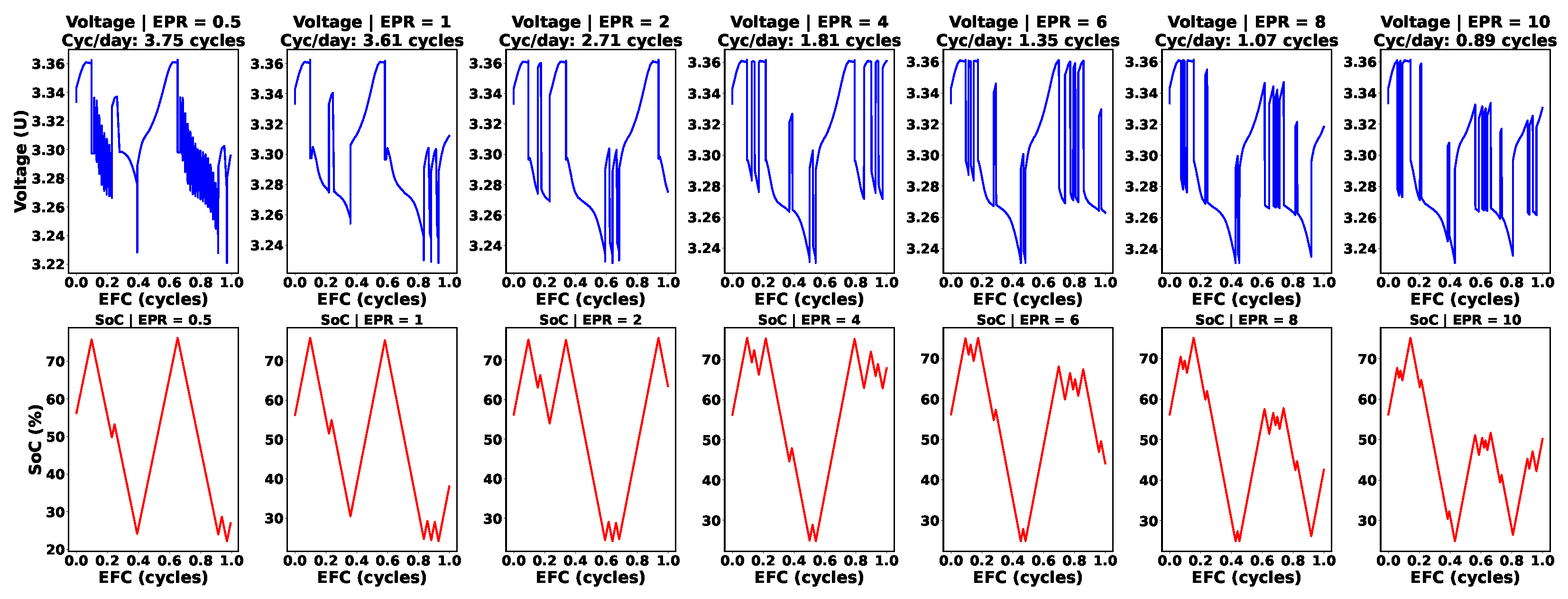
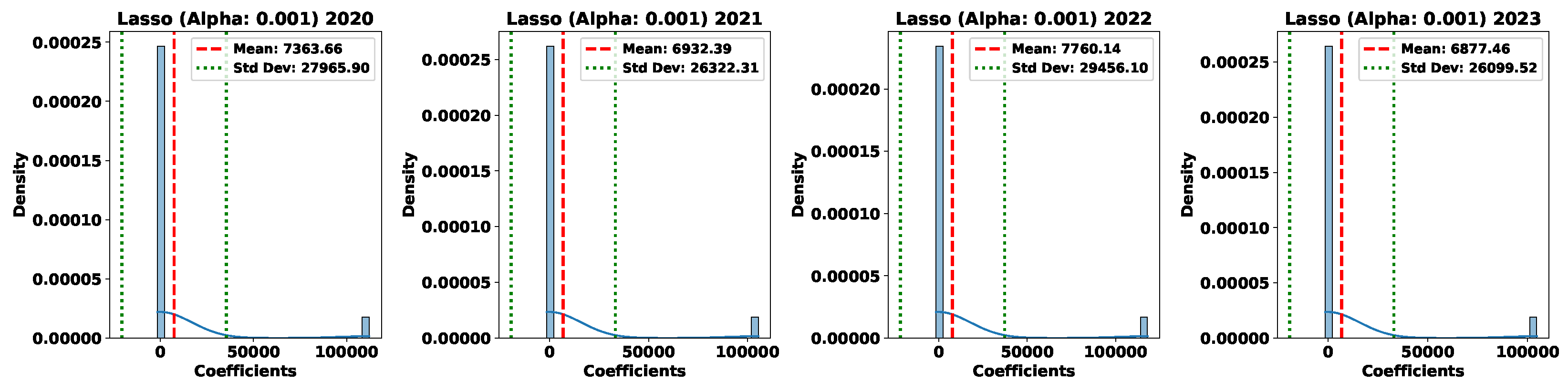
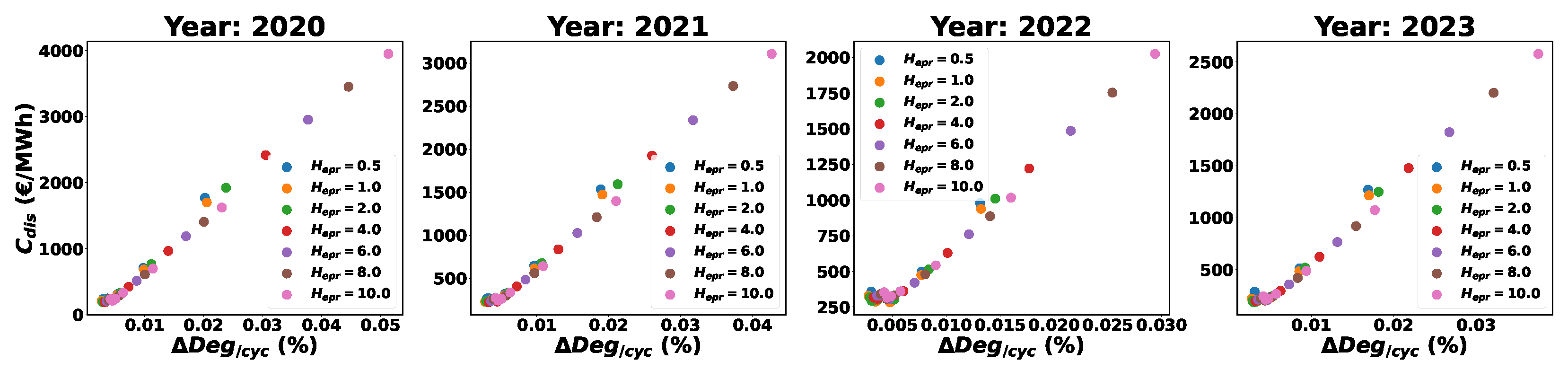
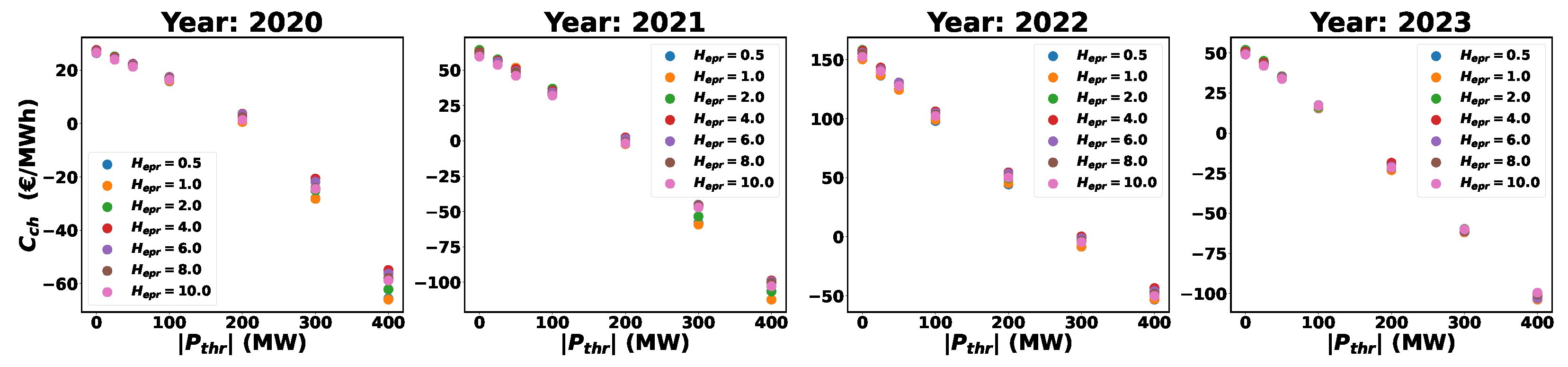
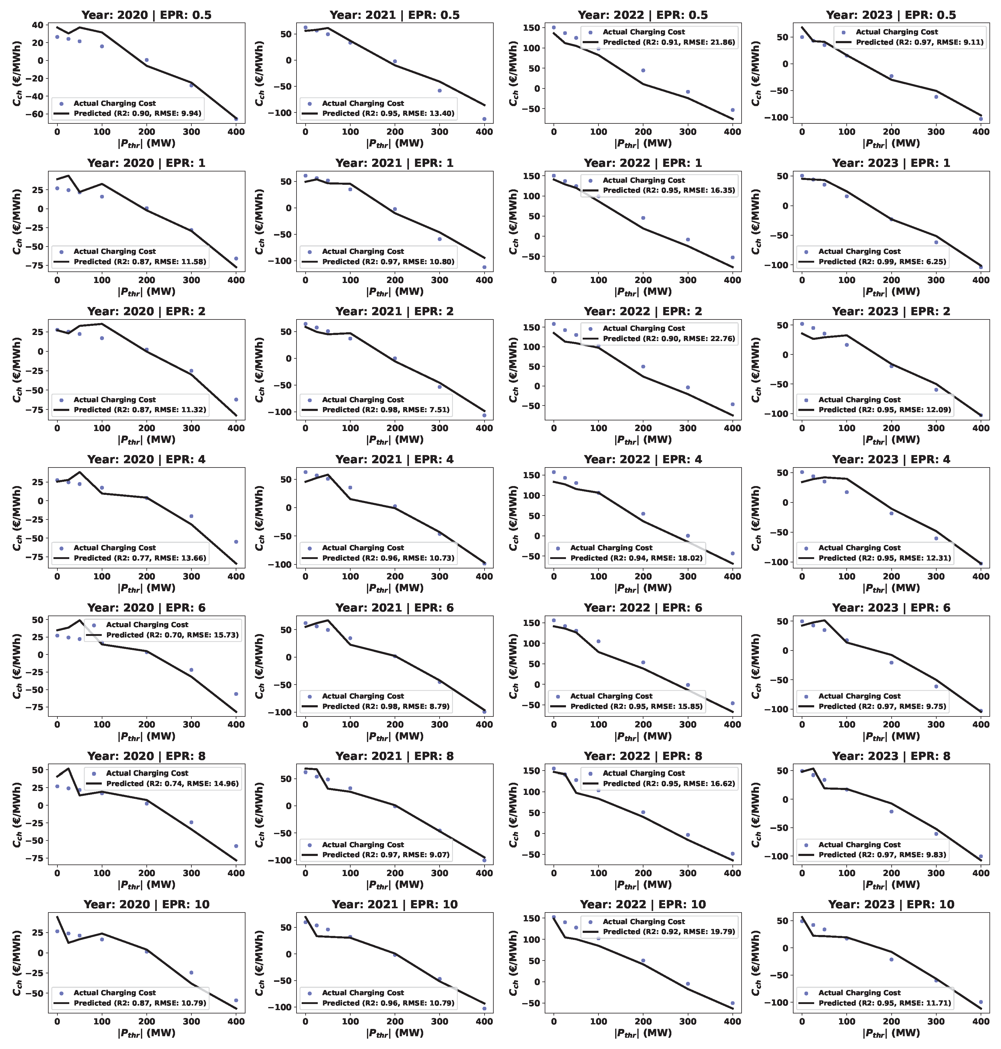
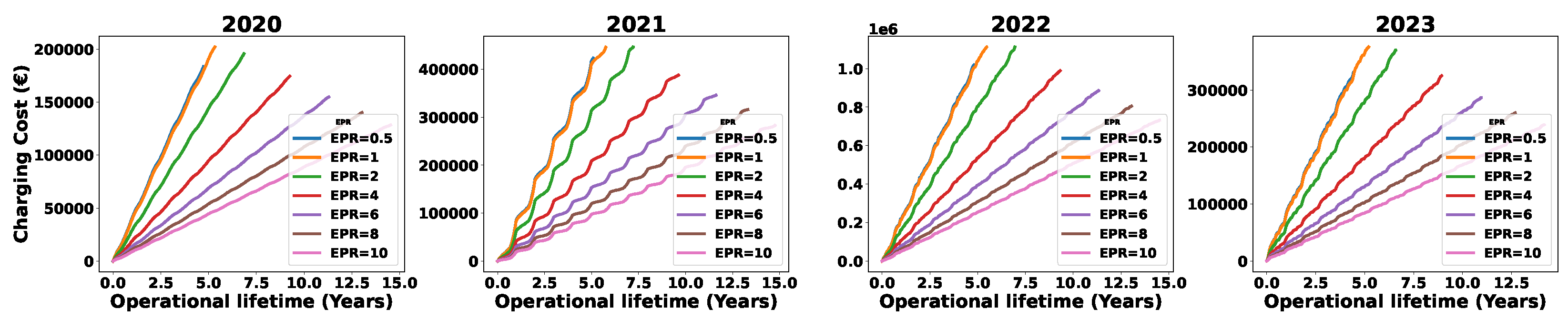
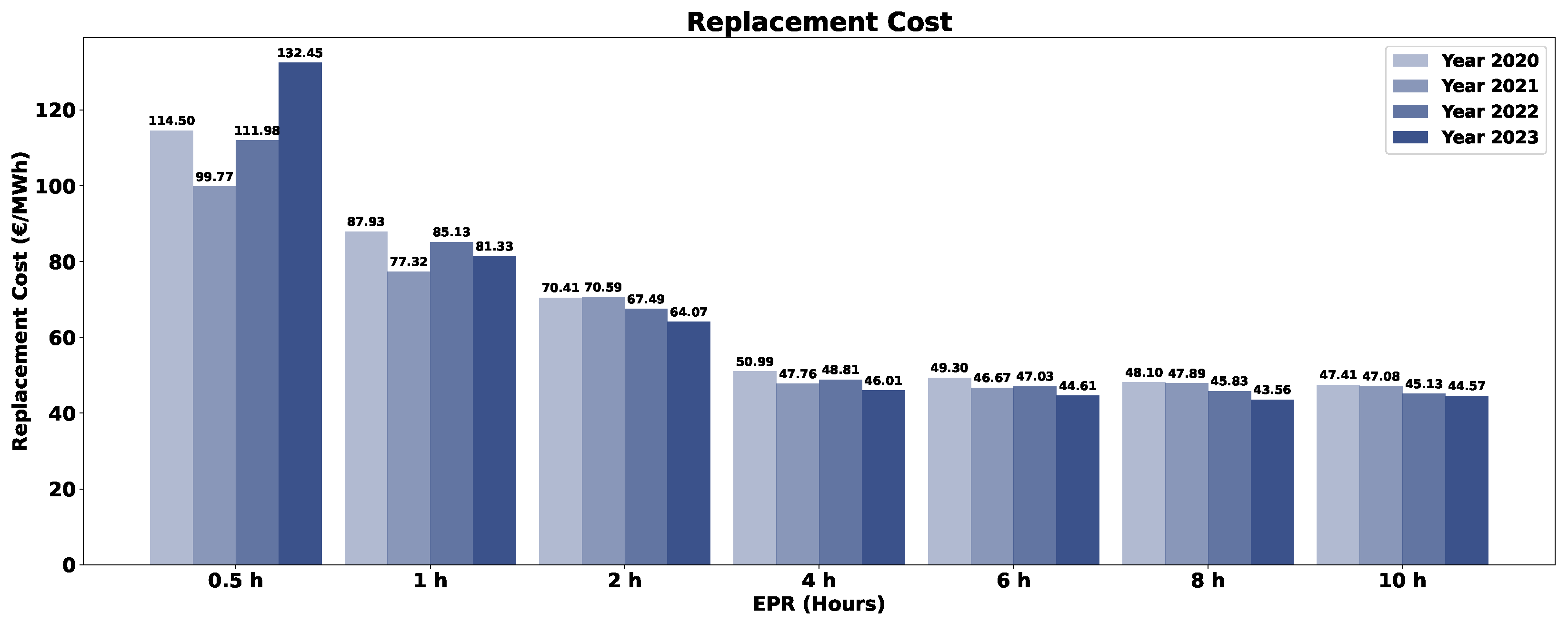
Table 1.
Detailed battery information parameters.
| Parameter | Value |
|---|---|
| Cell Voltage (Unom) | 3.2 V |
| Cell Voltage (Umin) | 2.8 V |
| Cell Voltage (Umax) | 3.65 V |
| Cell Capacity (Qini) | 50 Ah |
| State of Charge (SoCmin) | 25% |
| State of Charge (SoCmax) | 75% |
| State of Charge (SoCini) | 56.18% |
| State of Health (SoHeol) | 80% |
| Energy/Power Ratio (EPR) | 0.5, 1, 2, 4, 6, 8, 10 |
Disclaimer/Publisher’s Note: The statements, opinions and data contained in all publications are solely those of the individual author(s) and contributor(s) and not of MDPI and/or the editor(s). MDPI and/or the editor(s) disclaim responsibility for any injury to people or property resulting from any ideas, methods, instructions or products referred to in the content. |
© 2024 by the authors. Licensee MDPI, Basel, Switzerland. This article is an open access article distributed under the terms and conditions of the Creative Commons Attribution (CC BY) license (https://creativecommons.org/licenses/by/4.0/).
Share and Cite
MDPI and ACS Style
Ezennaya, S.O.; Kowal, J. Optimizing Energy Arbitrage: Benchmark Models for LFP Battery Dynamic Activation Costs in Reactive Balancing Market. Sustainability 2024, 16, 3645. https://0-doi-org.brum.beds.ac.uk/10.3390/su16093645
AMA Style
Ezennaya SO, Kowal J. Optimizing Energy Arbitrage: Benchmark Models for LFP Battery Dynamic Activation Costs in Reactive Balancing Market. Sustainability. 2024; 16(9):3645. https://0-doi-org.brum.beds.ac.uk/10.3390/su16093645
Chicago/Turabian StyleEzennaya, Samuel O., and Julia Kowal. 2024. "Optimizing Energy Arbitrage: Benchmark Models for LFP Battery Dynamic Activation Costs in Reactive Balancing Market" Sustainability 16, no. 9: 3645. https://0-doi-org.brum.beds.ac.uk/10.3390/su16093645
Note that from the first issue of 2016, this journal uses article numbers instead of page numbers. See further details here.