Advancing Spatial Drought Forecasts by Integrating an Improved Outlier Robust Extreme Learning Machine with Gridded Data: A Case Study of the Lower Mainland Basin, British Columbia, Canada

Abstract

Droughts have extensive consequences, affecting the natural environment, water quality, public health, and exacerbating economic losses. Precise drought forecasting is essential for promoting sustainable development and mitigating risks, especially given the frequent drought occurrences in recent decades. This study introduces the Improved Outlier Robust Extreme Learning Machine (IORELM) for forecasting drought using the Multivariate Standardized Drought Index (MSDI). For this purpose, four observation stations across British Columbia, Canada, were selected. Precipitation and soil moisture data with one up to six lags are utilized as inputs, resulting in 12 variables for the model. An exhaustive analysis of all potential input combinations is conducted using IORELM to identify the best one. The study outcomes emphasize the importance of incorporating precipitation and soil moisture data for accurate drought prediction. IORELM shows promising results in drought classification, and the best input combination was found for each station based on its results. While high Area Under Curve (AUC) values across stations, a Precision/Recall trade-off indicates variable prediction tendencies. Moreover, the F1-score is moderate, meaning the balance between Precision, Recall, and Classification Accuracy (CA) is notably high at specific stations. The results show that stations near the ocean, like Pitt Meadows, have higher predictability up to 10% in AUC and CA compared to inland stations, such as Langley, which exhibit lower values. These highlight geographic influence on model performance.

1. Introduction

Drought, a complex and least-understood natural disaster, has become increasingly prevalent in recent decades, necessitating effective management and resource preservation strategies [1,2]. The impacts of droughts on agriculture, water resources, ecosystems, and human settlements are severe and are escalating globally. Anthropogenic activities disrupting atmospheric dynamics contribute to drought events’ worsening frequency and intensity [3]. Mitigating these effects necessitates efficient early warning tools to aid rural communities in preparation [4]. Droughts, striking due to climatic factors, topography, and water demand, present a formidable challenge, causing economic, environmental, and social losses. Their prolonged duration demands accurate monitoring and forecasting, integrating meteorological and remote sensing data [5].

Predicting droughts is crucial for sustainable development and disaster risk reduction. Artificial intelligence (AI) methods, leveraging computational intelligence techniques, have proven powerful in forecasting meteorological time series and enhancing drought prediction capabilities [6,7,8,9]. AI’s contributions to environmental development, particularly in disaster risk management, are noteworthy [10]. In contrast to traditional models, AI models offer enhanced prediction accuracy by considering multiple variables and nonlinear relationships [11]. Anticipating droughts is significant in pre-emptive water resource management, agricultural strategizing, and disaster readiness. The progression of AI techniques has ignited a burgeoning enthusiasm for tapping into their potential to enhance Precision in drought prediction [10].

Dikshit et al. [12] conducted a study targeting drought prediction in New South Wales, Australia. They employed the Standardized Precipitation Evapotranspiration Index (SPEI) due to its comprehensive calculation, which considers temperature and rainfall, improving drought prediction. Utilizing climate research unit data, the index was constructed over varying periods (1, 3, 6, and 12 months). Their analysis incorporated 13 predictors, including sea surface temperature, climate factors, and diverse meteorological variables. Employing Artificial Neural Network (ANN) and Support Vector Machine (SVM) forecasting models trained on data from 1901 to 2010, they evaluated the models’ performance over eight years (2011–2018). The results demonstrated ANN’s superior performance (R² = 0.86) compared to SVM (R² = 0.75) in forecasting temporal drought patterns. Interestingly, the study unveiled the minimal influence of climatic indicators (e.g., Pacific decadal oscillation) and sea surface temperatures on temporal droughts. Zhang et al. [13] devised a distinctive drought forecasting model utilizing meteorological measurements, drought indices, and climatic signals from 32 stations in China’s Shaanxi Province. They employed cross-correlation function and distributed lag nonlinear model (DLNM) techniques to select predictors and ascertain their lag duration. DLNM, ANN, and XGBoost models were pitted against each other to forecast the SPEI for 1–6 months. The XGBoost model emerged as the frontrunner, exhibiting R² values of 0.68–0.95 across various lead times (3, 6, 9, and 12 months) and displaying superior accuracy in predicting overall, moderate, severe, and extreme droughts. Achite et al. [14] harnessed multiple Machine Learning (ML) techniques—ANN, ANFIS, SVM, and Decision Tree (DT)—for hydrological drought forecasting in the Wadi Ouahrane basin in Algeria. The authors assessed the models using evaluation metrics and found SVM to be the most effective in consistently accurately predicting hydrological droughts. Notably, the SVM model achieved a coefficient of determination of 0.95 for the 12-month timescale, showcasing its efficacy over varying time spans. Li et al. [15] explored a novel meteorological drought prediction strategy by incorporating antecedent SST fluctuation pattern (ASFP) and ML techniques like SVR, Extreme Learning Machine (ELM), and Random Forest (RF). They applied this approach to four drought-prone river basins globally, utilizing 1- and 3-month lead periods for forecasting SPEI. Their findings highlighted the ASFP–ELM model’s supremacy in predicting spatial-temporal drought evolution. Further research has delved into hybrid ML models fortified by optimization algorithms for enhanced drought prediction. Mohamadi et al. [16] harnessed SVM, Radial basis function network (RBFNN), ANFIS, and Multilayer perceptron (MLP) models to forecast climatic droughts in Iran using data spanning from 1980 to 2014. Incorporating the nomadic people algorithm (NPA), bat, salp swarm, and krill algorithms bolstered soft computing models’ accuracy and convergence speed. In their case, hybrid ML models exhibited improved performance, outperforming standalone models in forecasting the 3-month standardized precipitation index. Nabipour et al. [17] adopted an amalgamation of ANN models and optimization algorithms like the grasshopper optimization algorithm (GOA), salp swarm algorithm (SSA), particle swarm optimization (PSO), and biogeography-based optimization (BBO) for short-term hydrological drought prediction. Their hybrid models, particularly the ANN model coupled with the PSO algorithm, outperformed conventional ANN models, showcasing enhanced predictive accuracy for various drought indices at distinct time scales.

While droughts grip British Columbia, existing research lacks tailor-made ML tools for hydrological drought prediction. This study pioneers the Improved Outlier Robust Extreme Learning Machine (IORELM), a novel ML technique, to build robust forecasting models within the province. Unlike prior studies, IORELM goes beyond existing frameworks by meticulously analyzing various input combinations based on the Multivariate Standardized Drought Index (MSDI) to identify the most reliable model for predicting future droughts.

This novel approach promises to overcome current limitations in drought prediction, paving the way for significantly improved water management strategies. By enabling accurate forecasts, IORELM can empower the implementation of robust regulatory protocols and sustainable water use practices. This, in turn, bolsters mitigation efforts and safeguards water resources in British Columbia.

Moreover, this study breaks new ground by investigating the following:

• The efficacy of IORELM for drought forecasting: This represents the first application of IORELM to droughts in British Columbia, marking a significant step forward.
• Optimal input combinations: Analyzing various combinations based on MSDI parameters ensures the most reliable model is chosen, leading to improved prediction accuracy.
• Gridded reanalysis data in drought forecasting: This innovative approach has the potential to enhance prediction capabilities further.

By delving into these unexplored avenues, this study offers a groundbreaking approach to drought prediction in British Columbia, ultimately contributing to a more sustainable future for the province’s water resources.

2. Materials and Methods

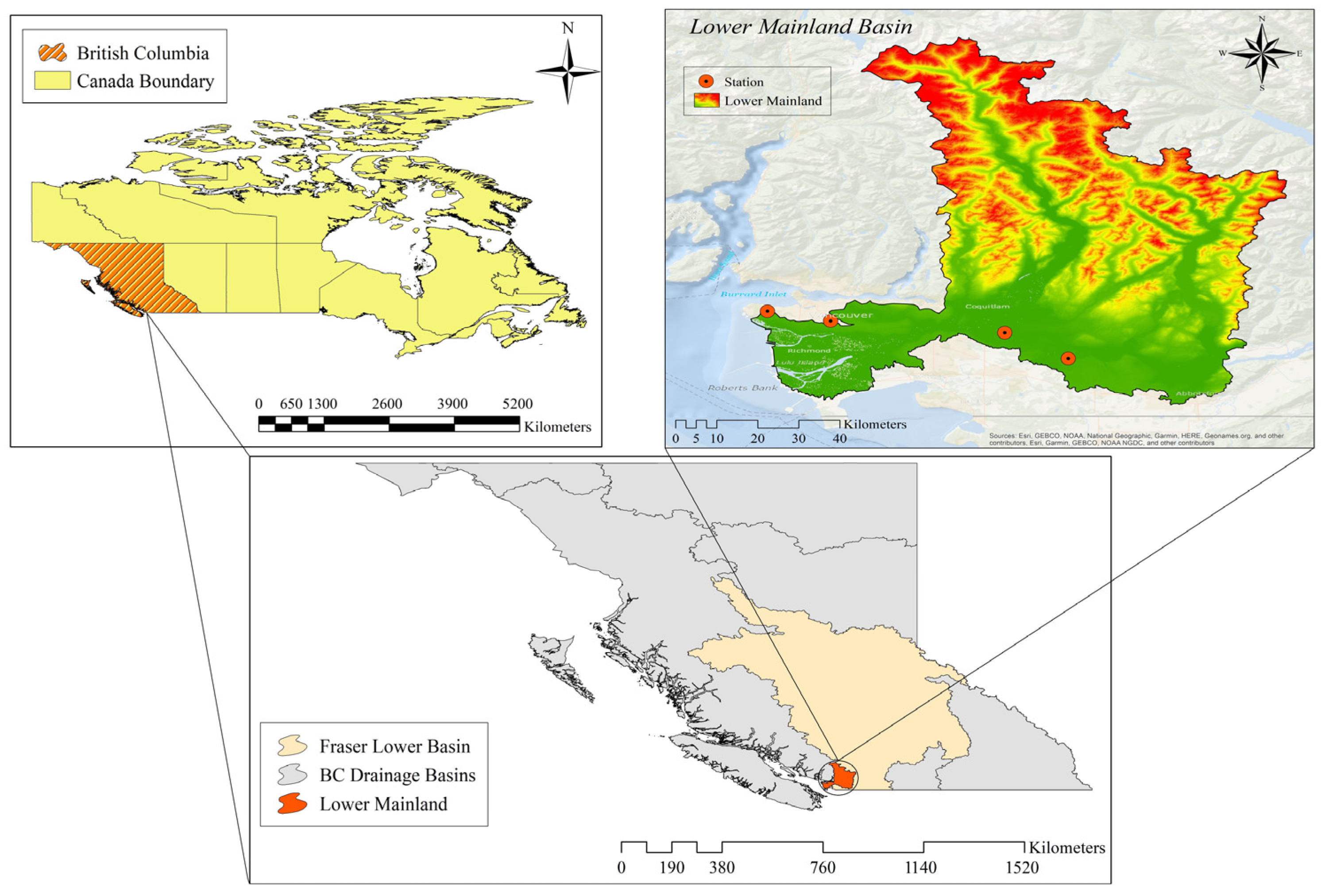
2.1. Study Area

The scope of our investigation is delimited to the Lower Mainland Basin within the province of British Columbia (B.C.), as visually outlined in Figure 1. This particular geographical area encompasses our primary research focus and serves as the backdrop for the placement and distribution of the monitoring stations essential to our study.

The British Columbia Drought Information Portal (DIP) reports a severe drought situation with a Drought Level 5—Adverse Impacts Almost Certain, signifying a critical water scarcity condition. This portal was established to serve as a comprehensive and centralized geographic information system for the residents of British Columbia. The DIP application employs a multifaceted approach, incorporating several embedded maps to provide users with valuable data related to drought conditions. The information available through the DIP encompasses various aspects, including the provincial drought levels, historical drought patterns over time, and supplementary drought-related details. Furthermore, it is important to note that the Drought Portal ensures that the drought levels and associated data are regularly updated promptly as new information becomes accessible through its website. In British Columbia, drought levels are typically assessed using a scale ranging from 0 to 5, with Drought Level 5 being the most severe and critical. This designation signifies that the likelihood of adverse impacts on communities and ecosystems is extremely high. As of the latest available data, which were recorded on September 21, it is observed that most of British Columbia’s water basins are currently experiencing Drought Levels 4 or 5, indicating a widespread and significant water shortage situation across the region [18]. Four meteoritical stations from Environment and Climate Change Canada (ECCC) were selected for the drought monitoring. The coordinates of this station are presented in

Table 1. Coordinates of the used stations.

Station	Latitude	Longitude
Lanfley	49°08′40.800″ N	122°33′03.600″ W
Pitt Meadows	49°12′29.964″ N	122°41′24.076″ W
Vancouver	49°17′43.270″ N	123°07′18.730″ W
West Vancouver	49°20′49.350″ N	123°11′35.910″ W

.

2.2. Data Acquisition

All the meteorological data are collected from the NCEP (National Centers for Environmental Prediction) and NCAR (National Center for Atmospheric Research). The NCEP/NCAR are collaborating on a significant project known as “reanalysis”. This project’s primary goal is to create a comprehensive 40-year record of global atmospheric field analyses to support the research and climate monitoring communities. This endeavor involves several crucial steps, including retrieving data from various sources such as land surface observations, ship records, rawinsonde (weather balloon) data, pibal observations (pilot balloons), aircraft data, satellite data, and more. These diverse data sources are subject to a rigorous quality control process. The collected data are incorporated into a consistent data assimilation system for the entire NCEP/NCAR 40-year project reanalysis period, using an advanced global system with a fixed configuration to avoid sudden climate data discontinuities. The database used in this project is as complete as possible, aiming to provide a comprehensive and accurate representation of atmospheric conditions over the specified time frame [19]. The NCEP operational Global Forecast System utilizes analysis and forecast grids with a global latitude–longitude grid resolution of 0.25 by 0.25 degrees. These grids encompass analysis and forecast time steps, following a pattern of a 3 h interval from 0 to 240 h and a 12 h interval from 240 to 384 h into the future. The model forecast runs occur at four specific Coordinated Universal Time (UTC) times daily, which are 00:00 UTC, 06:00 UTC, 12:00 UTC, and 18:00 UTC. This regular model run schedule ensures timely and up-to-date weather forecasting information for users and stakeholders [20]. For this research, the Precipitation and Soil moisture data were collected from 2019 to 2023 in a daily format.

2.3. Downscaling of Gridded Data

Downscaling methods, such as statistical and dynamical approaches, play a crucial role in providing higher-resolution climate information for local or regional applications. Statistical downscaling involves establishing relationships between large-scale atmospheric variables and local-scale climate conditions, utilizing techniques like regression models and weather generators. While computationally efficient, these methods may struggle to capture local-scale processes and extremes [2,9]. On the other hand, dynamic downscaling employs regional climate models to simulate climate at higher resolutions, considering regional-scale factors like topography and land use. Although offering detailed information on local-scale climate processes, dynamic downscaling requires intensive computation and careful calibration [21]. According to this, the collected data were downscaled using the Inverse Distance Weighting (IDW) technique as presented in Equation (1).

$$Z_u=\frac{{\displaystyle \sum \left(\frac{z_i}{d_i^p}\right)}}{{\displaystyle \sum \left(\frac{1}{d_i^p}\right)}}$$

(1)

where Z_u is the downscaled parameter in the desired location, Z_i is the known value (Precipitation and air temperature) at the sampled location i (sampled location), d_i is the distance between the un-sampled location (u) and each location (i), and p is a positive power parameter that determines the rate at which the weights decrease with distance. Common values for p include 1 (inverse linear distance weighting) and 2 (inverse squared distance weighting). In this study, p was 2. Following the downscaling process using the IDW technique, the derived values for each monitoring station were subsequently employed in the computation of the Drought Index specific to each station. This critical step allowed us to assess and quantify the drought conditions unique to each location under consideration. By utilizing the refined and downscaled data from both Precipitation and Soil Moisture sources, we could construct a localized Drought Index for every station.

2.4. The Multivariate Standardized Drought Index (MSDI)

The Multivariate Standardized Drought Index (MSDI) stands as a holistic drought assessment metric that embraces a multitude of factors, including precipitation, temperature, and streamflow, to evaluate drought conditions. Its comprehensive nature lies in considering the interconnectedness between various meteorological and hydrological elements [22]. Inspired by the widely adopted Standardized Precipitation Index (SPI), the prospect of formulating a multi-index model emerges by constructing a joint distribution function encompassing two or more univariate drought variables or indices. In this study, they introduce the MSDI, which extends the univariate SPI to incorporate the joint distribution of precipitation and soil moisture, a comprehensive approach for characterizing meteorological and agricultural drought. Central to this concept is copulas, a class of functions that enable the derivation of joint distributions for two or more variables, disregarding their original marginal distributions. They consider precipitation and soil moisture as random variables, represented as X and Y, respectively. The cumulative joint probability (p) can be succinctly expressed using a copula (C) as outlined in Equation (2). Copulas serve as mathematical tools enabling the derivation of the joint distribution of two or more variables, irrespective of their initial marginal distributions. They provide a means to model the interdependence or correlation between variables, allowing for a comprehensive understanding of their collective behavior within a given system [23]. By utilizing copulas, analysts and researchers can effectively capture the intricate relationships between variables, facilitating modeling. Furthermore, copulas offer a versatile framework that accommodates diverse types of data distributions, enabling the exploration of complex dependencies that may not be adequately captured by traditional statistical methods. Hence, their utilization represents a significant advancement in probability theory and statistical modeling, offering practitioners a powerful tool to analyze and interpret multivariate data effectively [23,24].

$$P\left(X<x,Y<y\right)=C\left(F_{\left(x\right)},G\left(Y\right)\right)=P$$

(2)

$$C\left(u,v\right)=-\frac{1}{\theta }\mathit{ln}\left(1+\frac{\left(e^{-\theta u}-1\right)\left(e^{-\theta v}-1\right)}{e^{-\theta }-1}\right)$$

(3)

$$\tau =1+\frac{4\left[D\left(\theta \right)-1\right]}{\theta }$$

(4)

$$D\left(\theta \right)=\frac{1}{\theta }{\displaystyle {\int }_0^{\theta }\frac{t}{exp\left(t\right)-1}dt}$$

(5)

$$MSDI={\phi }^{-1}\left(P\right)$$

(6)

In this context, C symbolizes the copula function, while F(X) and G(Y) refer to the marginal cumulative distribution functions of the random variables X and Y, respectively (see Equation (2)). The copula (C) introduces a dynamic framework for constructing the joint distribution of random variables while considering their individual marginal distributions. The integration of copulas in modeling nonlinear dependence structures within multivariate data has gained popularity in hydrological and climatological studies, encompassing applications such as multivariate frequency analysis, risk assessment, drought modeling, and geostatistical interpolation. Various copula families have been developed and employed to model diverse dependence structures of random variables. For instance, the Frank copula embodies a symmetric dependence structure, whereas the Gumbel and Clayton copulas manifest asymmetric dependence structures. For illustration, the Frank copula’s representation is as Equation (3). Here, θ signifies the parameter (drought), while u and v represent the marginal cumulative probabilities of precipitation and soil moisture, respectively. The parameter θ can be estimated via Kendall’s rank correlation “τ” in Equation (4). The function D(θ) is articulated as Equation (5), and “t” is the integration variable. Based on the cumulative joint probability “p” as depicted in Equation (2), the MSDI can be formulated as Equation (6). Here, $\phi$ embodies the standard normal distribution function. Equation (5) facilitates the conversion of the joint probability into the MSDI format, positioning it within the same realm as the original SPI, thereby enabling meaningful cross-comparisons across distinct drought indices. The methodology employed for SPI development can also be extended to other variables, such as soil moisture and runoff. Using copulas facilitates a cohesive representation of the interrelationship between precipitation and soil moisture, transcending the boundaries of their marginal distributions. This innovative approach, embodied by the MSDI, showcases the potential for a more holistic understanding of meteorological and agricultural drought dynamics [22]. The MSDI is pivotal in drought monitoring, early warning systems, and decision making across diverse domains such as agriculture, water resource management, and disaster preparedness. By embracing multiple variables, it offers a more comprehensive and unified viewpoint of drought conditions, capturing intricate interactions between meteorological and hydrological dynamics. However, it is imperative to underline that accurate MSDI calculation necessitates dependable and quality-assured data for all involved variables. Additionally, selecting variables, corresponding weights, and the methodology employed in analysis can influence outcomes and interpretations. A meticulous approach and validation are indispensable when applying the MSDI in practical contexts and policy formulation [24].

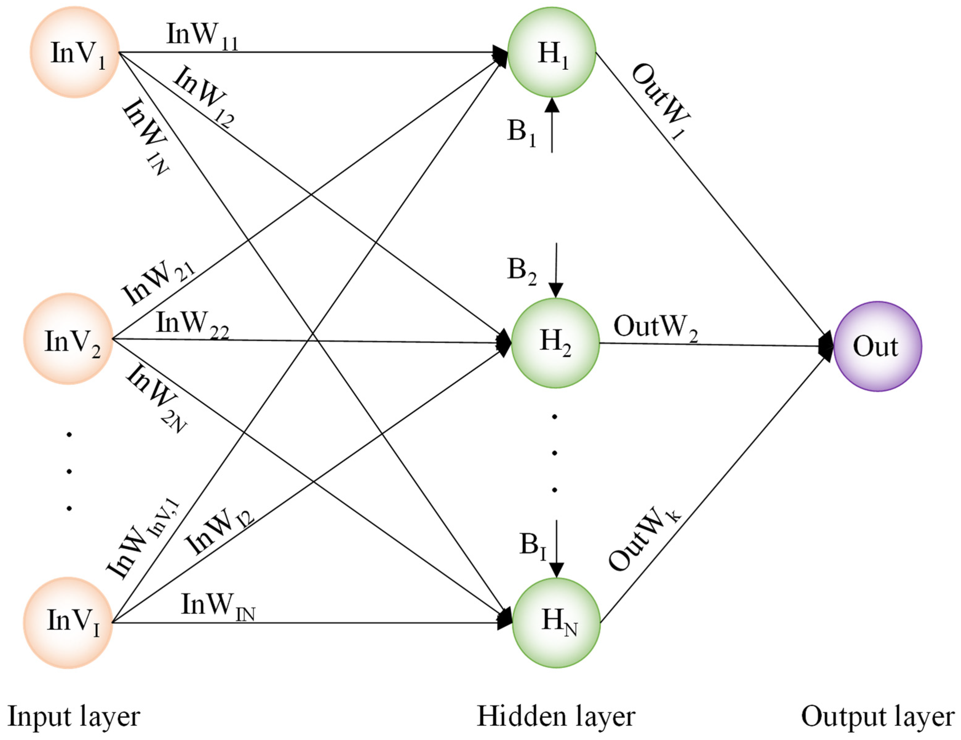
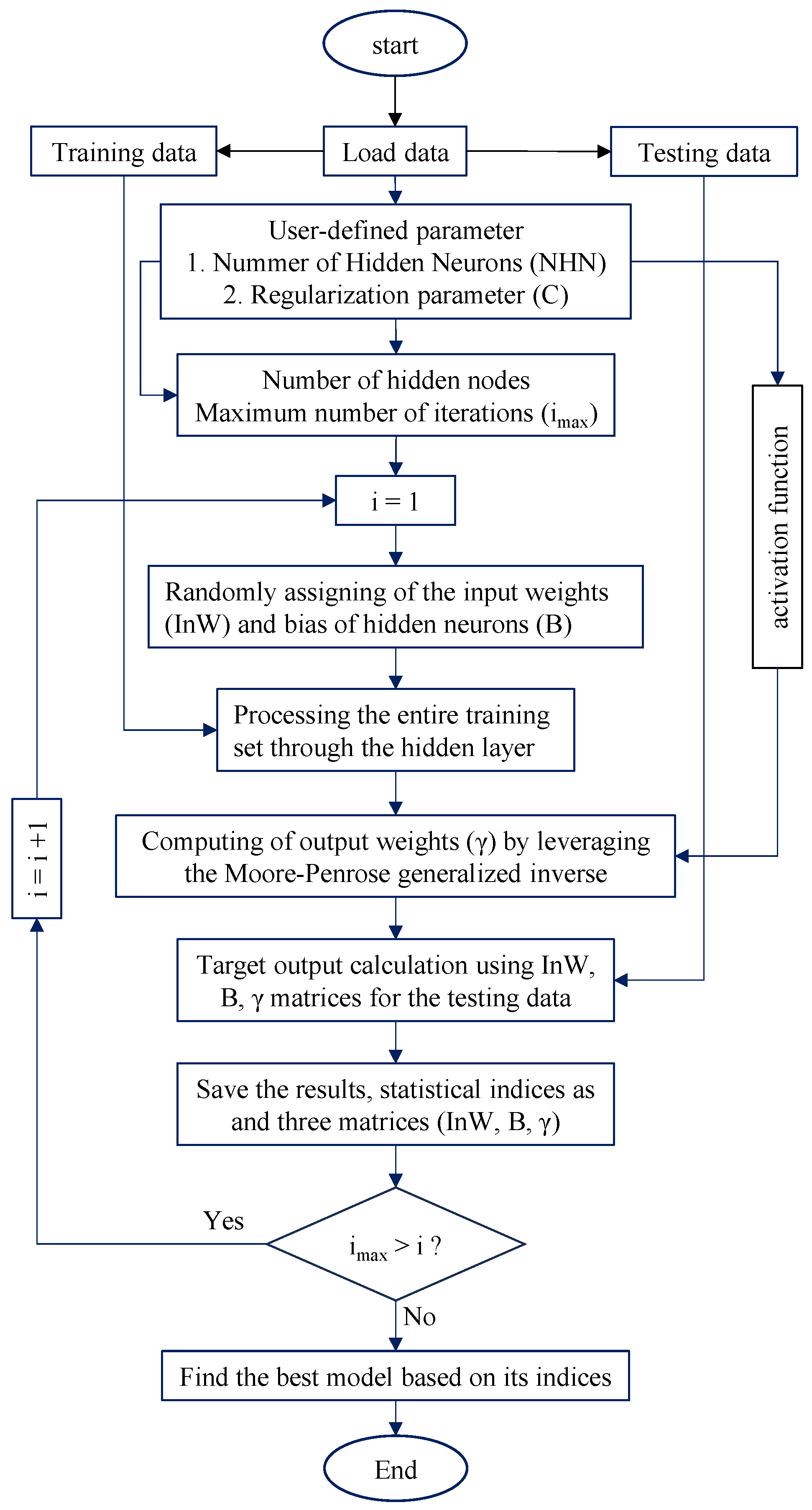
2.5. Improved Outlier Robust Extreme Learning Machine (IORELM)

Extreme Learning Machine (ELM) is a learning algorithm for single-hidden layer feedforward neural networks (SLFFNNs) that was introduced by Guang-Bin Huang and colleagues in the early 2000s [25,26]. ELM is designed to overcome some of the difficulties and limitations associated with traditional feedforward neural network training methods, such as slow training speed [27], local minima [28,29], and the need for the iterative tuning of learning parameters [30].

ELM is primarily characterized by its extremely fast learning speed and ease of implementation [31]. It randomly assigns input weights and biases and analytically determines the output weights of SLFFNNs. This approach eliminates the need for iterative adjustment, making the learning process significantly faster than conventional gradient-based learning methods. A schematic of the ELM structure is presented in Figure 2.

The key idea behind ELM is to randomly choose hidden nodes’ input weights and biases and calculate the output weights analytically. The initial phase involves randomly allocating weights and biases for inputs. During this stage, each pair in the training dataset, denoted as (xⁱ, yⁱ)—where xi represents the input vector and yⁱ the desired output—is processed by assigning random values to the input weights (InW) (Equation (7)) and biases (B) (Equation (8)) of the nodes within the hidden layer.

$$InW={\left[\begin{array}{ccc}In{W}_{11}& \cdots & In{W}_{I1}\\ ⋮& \ddots & ⋮\\ In{W}_{N1}& \cdots & In{W}_{NI}\end{array}\right]}_{N\times I}$$

(7)

where N represents the number of neurons in the hidden layer, while i indicates the number of input variables.

$$B={\left[\begin{array}{c}{B}_1\\ ⋮\\ B_N\end{array}\right]}_{N\times 1}$$

(8)

The second phase entails computing the hidden layer’s output matrix (K). For every input sample, the hidden layer’s output is derived through an activation function, culminating in the formation of the hidden layer output matrix K. For detailed information on various activation functions, refer to the studies in the literature [30].

In the third phase, the focus shifts to establishing the output weights (γ) that link the hidden layer with the output layer. These weights are determined analytically by identifying the least squares solution to the following linear equation.

$$\mathbf{K} \gamma =\mathbf{Y}$$

(9)

where

$$\mathbf{Y}={\left[\begin{array}{c}{y}_1^T\\ ⋮\\ y_n^T\end{array}\right]}_{n\times 1}$$

(10)

$$\gamma ={\left[\begin{array}{c}{\gamma }_1^T\\ ⋮\\ {\gamma }_N^T\end{array}\right]}_{N\times 1}$$

(11)

$$\mathbf{K}={\left[\begin{array}{ccc}f(In{W}_1\cdot x_1+B_1)& \cdots & f(In{W}_N\cdot x_1+B_N)\\ ⋮& \ddots & ⋮\\ f(In{W}_1\cdot x_n+B_1)& \cdots & f(In{W}_N\cdot x_n+B_N)\end{array}\right]}_{n\times N}$$

(12)

where n denotes the number of training samples, N represents the count of neurons in the hidden layer, InW refers to the matrix of input weights, B indicates the bias associated with the hidden neurons, x is the set of input variables, Y stands for the matrix of target outputs, and γ signifies the output weight.

An effective approach to addressing this issue involves determining the best value for $\widehat{\gamma }$ by minimizing the loss function, which is achieved through calculating the optimal least squares.

$${\mathrm{E}}_{\mathrm{ELM}}=min‖\mathbf{y}-\mathbf{K}\gamma ‖$$

(13)

This process typically involves employing the Moore–Penrose generalized inverse of matrix K, denoted as K⁺, resulting in the following equation in the sense of minimum ℓ2-norm to find the optimal output weights.

$$\widehat{\gamma }={\mathrm{K}}^{+}\mathrm{Y}$$

(14)

The crucial aspect of ELM lies in forming a specific matrix by minimizing training errors, which is significantly influenced by the random assignment of input weights and biases to hidden neurons. Bartlett [32] highlighted that in an FFNN, maximum generalization capability is achieved when both the training error and the magnitude of output weights are minimized concurrently. Similarly, optimal generalization is realized in ELM by striking the right balance between minimizing the output weights’ norm and the training error [32]. A regularization parameter (C) is employed to enhance the ELM’s ability to generalize beyond the training data to find this balance. Introducing this parameter is meant to improve the model’s performance on new, unseen data, thereby extending the capabilities of the standard ELM approach.

The training error (e = y − Kγ) can be treated as a measure of sparsity to improve the modeling effectiveness when outliers are present. The ℓ0-norm more accurately represents the sparsity compared to the ℓ2-norm [33]. Detailed information about sparsity can be found in Bonakdari et al. [30]. ORELM aims to find an output weight (γ) with a minimal ℓ2-norm, ensuring that the training error remains sparse. The loss function of the ORELM is defined as follows:

$${\mathrm{E}}_{\mathrm{ORELM}}=\underset{\gamma }{\mathrm{C}min}{‖\mathbf{y}-\mathbf{K}\gamma ‖}_0+{‖\gamma ‖}_2^2$$

(15)

The output weight is calculated using the following equations [30]:

$${\beta }_{k+1}={({\mathbf{K}}^T\mathbf{K}+2/C\mu \mathbf{U})}^{-1}{\mathbf{K}}^T(\mathbf{y}-{(\mathbf{e})}_{\mathsf{k}}+{\lambda }_k/\mu )$$

(16)

$$\begin{array}{ll}{\mathbf{e}}_{\mathrm{k}+1}=& \mathrm{shrink}(\mathbf{y}-\mathbf{K}{\gamma }_{\mathrm{k}+1}+{\lambda }_{\mathrm{k}}/\mu ,1/\mu )\\ & \cong max\left\{\left|\mathbf{y}-\mathbf{K}{\gamma }_{\mathrm{k}+1}+{\lambda }_{\mathrm{k}}/\mu \right|-1/\mu ,0\right\}\circ \mathrm{sign}\left(\mathbf{y}-\mathbf{K}{\gamma }_{\mathrm{k}+1}+{\lambda }_{\mathrm{k}}/\mu \right)\end{array}$$

(17)

$${\lambda }_{\mathrm{k}+1}={\lambda }_{\mathrm{k}}+\mu \left(\mathbf{y}-\mathbf{K}{\gamma }_{\mathrm{k}+1}-{\mathbf{e}}_{\mathrm{k}+1}\right)$$

(18)

where $\mu =2\mathrm{n}/{‖\mathbf{y}‖}_1$, and U is the unit matrix.

Ebtehaj and Bonakdari [34] highlighted that over two-thirds of the adjustable parameters in the ORELM consist of the input weights and biases of hidden neurons, which are generated randomly and greatly influence the model’s outcomes [34]. Incorrect settings for these parameters can diminish the model’s ability to generalize. To address this, the study introduces two enhancements to the standard ORELM: (1) the implementation of an orthonormal basis for the distribution of input weights and bias within the hidden neuron matrices and (2) the inclusion of an iteration parameter. These modifications led to an enhanced version of ORELM, termed Improved ORELM (IORELM). The process for this refined model, IORELM, is depicted in Figure 3.

The modeling process begins with the initialization phase, where the structure of the IORELM is outlined, specifying the number of hidden nodes and randomly assigning input weights and biases to these nodes. In this study, the maximum number of iterations and number of hidden neurons were considered as the maximum value that can be taken. These values were calculated using Equation (19) [31].

$$MaX\_NHN=Training samples/(InV+2)$$

(19)

where MaX_NHN is the maximum number of allowable hidden neurons, and InV is the number of input variables.

For the regularization parameter, the optimal value was determined to be 0.1 based on iterations. This value was found to provide the best balance between fitting the training data well and avoiding overfitting, resulting in improved generalization performance on unseen data [34].

Following this, the forward pass phase involves processing the entire training set through the hidden layer, utilizing the randomly determined weights, biases, and a chosen activation function to compute the outputs of the hidden layer. Subsequently, output weights are determined by leveraging the Moore–Penrose generalized inverse to address the least squares problem, ensuring the output weights are optimally aligned with the desired outcomes. In the testing and validation phase, test data are passed through the established hidden layer—retaining the initially set weights and biases—and then through the output layer, employing the calculated output weights to generate predictions.

The final stage focuses on assessing the IORELM model’s efficacy, thereby quantifying its performance and capability to generalize over unseen data. From initialization to performance evaluation, this comprehensive approach encapsulates the ELM’s modeling process, emphasizing systematic progression and rigorous validation to ensure the model’s robustness and effectiveness.

Following this, the outcomes of each iteration are recorded, and the process is repeated for the predetermined maximum number of iterations. Subsequently, the most optimal model is selected based on the computed statistical indices, concluding the iterative and evaluative phases of the IORELM modeling process.

2.6. Metrics for Assessing the Performance of Methods

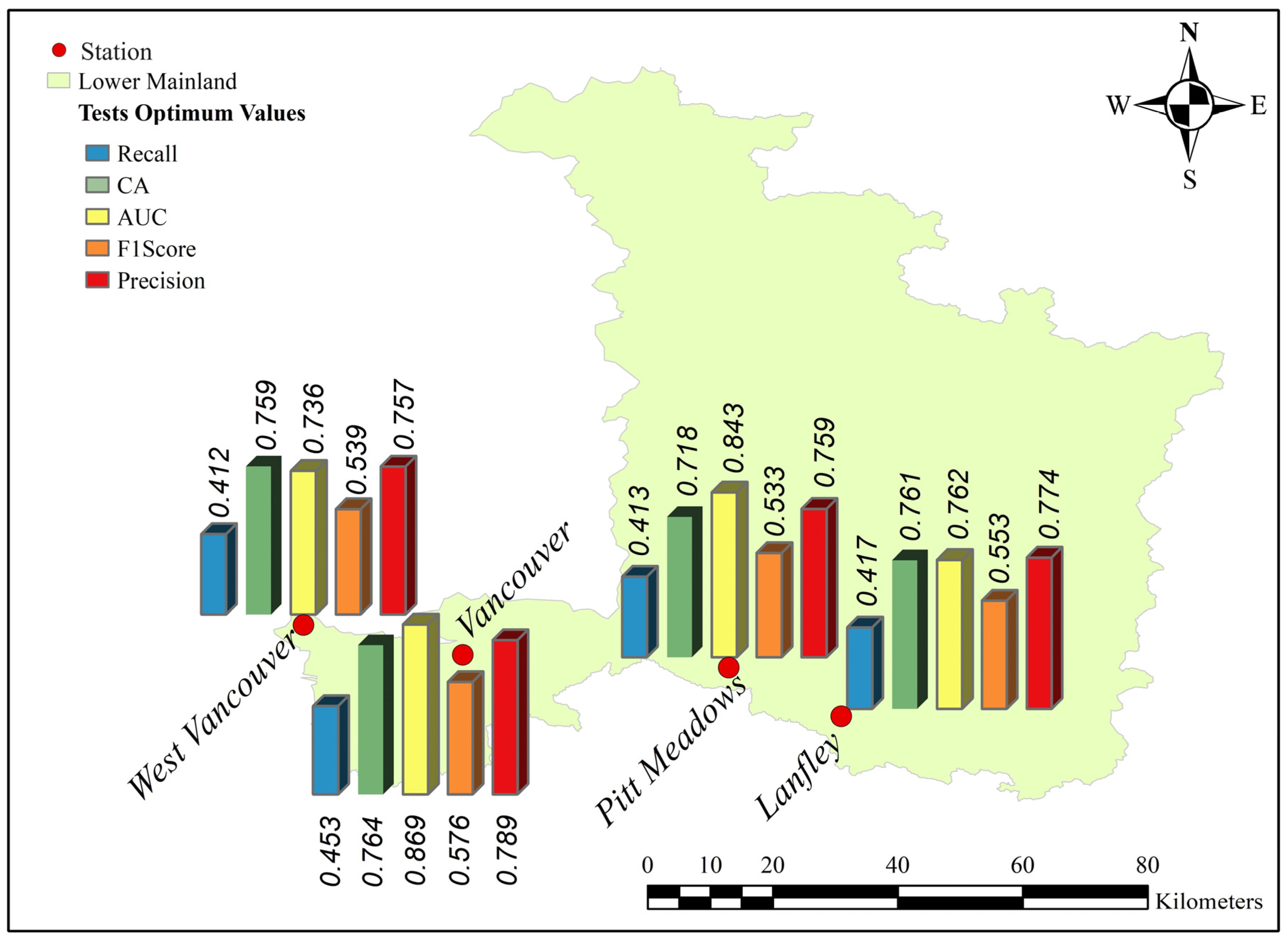
In this study, we assess the efficacy of the proposed techniques for Drought estimation. The development and deployment of binary classification models demand a comprehensive understanding of their performance, often evaluated using metrics such as Precision, Classification Accuracy (CA), Recall, Area Under the Curve (AUC), and F1-Score [35].

Precision (Equation (20)) measures the proportion of true positive predictions out of all positive predictions, indicating the model’s ability to avoid false positives [36].

Classification Accuracy (Equation (21)) assesses the overall correctness of the model’s predictions by comparing the number of correctly predicted instances to the total number of instances. Recall (Equation (22)), also known as sensitivity, evaluates the proportion of true positive predictions out of all actual positives, indicating the model’s ability to identify all relevant instances [2,37].

The F1-Score (Equation (23)) also harmonizes Precision and Recall, offering a balanced measure of the model’s overall accuracy by considering both false positives and false negatives. Understanding these performance metrics is crucial for effectively developing, evaluating, and deploying binary classification models in diverse real-world applications [38].

$$\mathrm{Precision}=\frac{\mathrm{True} \mathrm{Positive}}{\mathrm{True} \mathrm{Positive}+\mathrm{False} \mathrm{Positive}}$$

(20)

$$\mathrm{Recall}=\frac{\mathrm{True}\mathrm{Positive}}{\mathrm{True} \mathrm{Positive}+\mathrm{False} \mathrm{Negative}}$$

(21)

$$\mathrm{Accuracy}=\frac{\mathrm{Number} \mathrm{of} \mathrm{Correct} \mathrm{Predictions}}{\mathrm{Total} \mathrm{Number} \mathrm{of} \mathrm{Predictions}}$$

(22)

$$\mathrm{Fl}\mathrm{Score}=\frac{\mathrm{Precision}+\mathrm{Recall}}{\mathrm{Precision}\times \mathrm{Recall}}$$

(23)

In binary classification, four potential prediction outcomes may arise [39]. “True positive” signifies accurately predicting the presence of drought, indicating that the model correctly identifies instances of drought. “True negative” denotes the correct prediction of the absence of drought, meaning the model accurately identifies instances where drought does not occur. Conversely, a “false positive” occurs when the model incorrectly predicts drought when none is present, leading to a false alarm. Similarly, a “false negative” arises when the model fails to predict drought when it does occur, indicating a missed detection. These four outcomes are essential for evaluating the performance and reliability of binary classification models, particularly in domains where accurate identification of positive and negative instances is critical, such as drought prediction and mitigation efforts [40].

AUC measures the ability of the model to discriminate between positive and negative instances across various threshold values. It plots the true positive rate (sensitivity) against the false positive rate (1-specificity) and provides a single scalar value representing the model’s performance [41].

3. Results

Following the methodology outlined in reference [30,31,34], the SPI and standard soil moisture index (SSI) are computed using the corresponding precipitation and soil moisture datasets. To investigate the MSDI across a time scale (daily), SPI and SSI are calculated for identical durations to allow for cross-comparison. Across various grid areas, three copula functions (Frank, Gumbel, and Clayton) are selected, as these copula functions are commonly employed in drought studies [42,43,44].

The effectiveness of different copula models in accurately representing the relationship between rainfall and soil moisture. Among the options, Gumbel Copula emerges as the preferred choice for the majority of cases, as presented by Masud et al. [45]. A copula model is retained if its corresponding p-value is equal to or higher than 0.05 (5% significance level). These tests are conducted to maintain consistency with SPI and SSI analyses.

In this study, a total of 14 inputs, as outlined in

Table 2. Description of the different inputs for ML.

Input Name	Description
P(t)	Total Precipitation
P(t − 1)	1-day lag of total precipitation
P(t − 2)	2-day lag of total precipitation
P(t − 3)	3-day lag of total precipitation
P(t − 4)	4-day lag of total precipitation
P(t − 5)	5-day lag of total precipitation
P(t − 6)	6-day lag of total precipitation
SM(t)	Soil moisture
SM(t − 1)	1-day lag of soil moisture
SM(t − 2)	2-day lag of soil moisture
SM(t − 3)	3-day lag of soil moisture
SM(t − 4)	4-day lag of soil moisture
SM(t − 5)	5-day lag of soil moisture
SM(t − 6)	6-day lag of soil moisture

, were utilized in various combinations. The total number of data for each input was 1523. The data were sufficient for drought prediction using the ML technique [10,40]. These inputs generated a comprehensive dataset comprising 16,383 distinct combinations for modeling purposes. Among these inputs, a primary focus was placed on two key parameters of MSDI, which encompassed precipitation (P(t)) and soil moisture (SM(t)) variables. These parameters were derived using a range of lag intervals, spanning from a one-day lag to a six-day lag (P(t − i) and SM(t − i)). This study aimed to capture varying temporal relationships between the input variables and target outcomes by incorporating different lag intervals. This extensive exploration of input combinations facilitated a thorough examination of the predictive performance of ML models across a diverse array of environmental conditions and temporal contexts.

The modeling process involved classifying MSDI values for four distinct stations using different combinations of the inputs listed in Table 2. In this table, P(t − i) shows the ith lag of the total precipitation, and SM(t − i) is the ith lag of the soil moisture. These combinations ranged from utilizing as few as one input to incorporating all 14 inputs simultaneously. Each input represents a specific variable relevant to the MSDI, such as precipitation and soil moisture, with variations in time intervals captured through lag intervals ranging from one month to six days. By exploring these diverse input combinations, the study aimed to comprehensively analyze how different combinations of variables and temporal relationships influence the classification of MSDI values across the four stations. This approach allowed for a thorough examination of the predictive capabilities of the ML models under various scenarios, enabling insights into the most influential factors impacting MSDI classification across different spatial and temporal contexts.

To assess the performance of ML classification considering the best statistical sets of inputs and evaluate how efficiently these models can predict the MSDI drought index using precipitation and soil moisture data, we applied five evaluation tests (Precision, CA, Recall, AUC, and F1-Score). Here is a brief explanation of each of the five-evaluation metrics used.

Precision metric measures the proportion of positive identifications that were actually correct. It is the number of true positives divided by the total number of positive predictions (the sum of true positives and false positives) [46]. Recall (Sensitivity) assesses the proportion of actual positives that were identified correctly. It is calculated by dividing the number of true positives by the sum of true positives and false negatives [47]. This metric is critical when the cost of missing a true positive is significant. The F1-Score is the harmonic mean of Precision and Recall [48]. It conveys the balance between the precision and recall metrics, providing a single score that reflects the robustness of the model’s ability to classify positive instances correctly. It is particularly useful when one needs to take both false positives and false negatives into account. CA is the overall percentage of correct predictions, both true positives and true negatives, among the total number of cases examined [49]. It is the most intuitive performance measure, simply a ratio of correctly predicted observations to the total observations. AUC provides an aggregate measure of performance across all possible classification thresholds. It measures the ability of the model to discriminate between positive and negative classes [50]. An AUC of 1 indicates perfect prediction, while an AUC of 0.5 suggests no discriminative power [51]. Moreover, the optimum results of all five tests for the four stations in the study area were also evaluated, which allowed for a comprehensive assessment of the accuracy of the classification results.

In the following section, the evaluation of each test result for the four stations situated within the study area is depicted in Figure 4. These figures provide a comprehensive overview by presenting the average value of each metric derived from the modeling during the test phase. Each station’s performance is discussed separately, allowing for a detailed analysis of the model’s efficacy across various locations within the study area.

From the results of the precision test for the four stations based on Figure 4a, we can deduce that the Pitt Meadows station has the highest precision score, suggesting that, for that specific station, the model made the most relevant classifications out of the four. The lowest precision score is for the West Vancouver station, suggesting it had relatively more false positives or fewer true positives in comparison to the others.

Regarding the location of these stations within the study area and the effects of proximity to different geographical features, such as the ocean (to the southwest) or moving north or south within the basin, those stations closer to the ocean may be influenced by more stable and higher humidity conditions due to the proximity of the water body. This could potentially affect the MSDI drought index because factors like precipitation and soil moisture may have different patterns near coastal areas versus inland areas [52,53]. Moreover, stations located in the northern part of the study area might experience different weather patterns influenced by the terrain and distance from the ocean, which could result in variations in precipitation and soil moisture levels. Similarly, these factors could also affect areas in the southern part of the case study, along with potential human activities that might influence local climate conditions.

To evaluate the average results of the CA test values for the four stations, we analyzed Figure 4b, which represents the average of the provided CA values. The average CA value for the four stations is approximately 0.702. A higher average CA would indicate that the model has a good overall prediction rate [54]. However, it is essential to note that while high CA is desirable, it is not the only metric to consider, especially in datasets that might have an imbalance between classes. Other metrics like Precision, Recall, F1 score, and AUC can provide a more nuanced understanding of the model’s performance, especially in terms of its ability to handle false positives and false negatives.

With the provided CA values, we can see that they are high, suggesting that the model has a decent prediction capability across the study area for the MSDI drought index, which uses precipitation and soil moisture as inputs [55]. It would also be beneficial to look at the other metrics to obtain a comprehensive view of the model’s performance.

In Figure 4c, AUC represents a degree of separability. It indicates how much the model is capable of distinguishing between classes. Higher AUC values typically indicate better model performance [50]. The average AUC value for the four stations is 0.745. For the analysis of the AUC values in relation to the geographic location of the stations, stations closer to the ocean (West Vancouver and Vancouver stations) have higher AUC Values. This means coastal regions may have more consistent patterns of precipitation and soil moisture due to marine influence. This could lead to a more consistent signal in the data from which the ML model can learn, potentially resulting in higher AUC values. Hence, a higher AUC value indicates better separability between classes, suggesting that the model can distinguish well between drought and non-drought conditions. This could be due to the clearer patterns in climatic data near the coast.

In addition, stations closer to the North or South (away from the ocean), might present more varied AUC values due to diverse microclimates and a wider range of influences on precipitation and soil moisture, such as elevation, terrain, and distance from moderating oceanic effects. In summary, the AUC values suggest that the classification model is fairly good at distinguishing between classes across the stations in the study area. The minor differences in AUC values may reflect the subtle influences of local geography and climate. The model must be trained on diverse data that capture the full spectrum of conditions across the study area to maintain high performance in all locations.

Figure 4d includes the Recall test values for four stations within the study area, the Lower Mainland Basin in British Columbia. The average Recall value for the four stations is approximately 0.361. For the analysis of the Recall values in relation to the geographic location of the stations, stations closer to the ocean (West Vancouver and Vancouver stations) have more predictable moisture patterns due to the proximity to large bodies of water, which could lead to higher Recall as the model may better identify actual drought events. However, suppose drought patterns are less common because of the marine climate. In that case, the Recall might be lower since there are fewer drought events to identify, which can affect the model’s ability to learn from such events. Furthermore, those stations away from the ocean may experience more variable weather patterns and potentially have less predictable soil moisture levels due to terrain and elevation, leading to a lower Recall if the model fails to identify all positive cases.

Alternatively, consider a situation where drought occurrences are more frequent, and the model has been adequately trained on a substantial dataset that accurately represents these conditions. This means that the model has been exposed to ample instances of drought events during its training phase. As a result, it possesses a thorough understanding of the patterns and characteristics associated with droughts. This enhanced training enables the model to better predict and analyze drought-related phenomena, offering valuable insights into their causes, impacts, and potential mitigation strategies. In that case, the Recall might be higher as the model would have learned to identify the signs of drought more effectively. The relatively low Recall values across the stations suggest that the model may be missing a significant number of actual drought events. This could be due to a variety of factors, including imbalanced datasets (where the number of non-drought events far exceeds drought events), insufficient representation of drought characteristics in the features used for training, or complex interactions between climatic variables that the model is not capturing [56].

Figure 4e includes the F1-Score test values for four stations within the study area. The average F1-Score value for the four stations is approximately 0.583. Considering Figure 4e, stations closer to the ocean have more consistent and measurable precipitation and soil moisture patterns due to the marine influence, leading to clearer patterns for the ML model to learn from. This could potentially result in higher F1-Scores due to better model precision and Recall.

As the primary visual tool in this current study, violin plots have been used to show the distribution of the index values regarding all stations and models. This decision is underpinned by the plots’ unique ability to provide a comprehensive overview of the data, merging the insights into central tendencies and dispersion, characteristic of box plots, with the distributional shape information offered by density plots [28,29]. The depiction of density estimates on both sides of the central box plot is especially valued, revealing potential multimodality or skewness in the data—a nuanced detail that might remain hidden under alternative plotting methods. Such a feature is deemed invaluable in the comparative analysis across multiple groups of models, where discerning and illustrating distributional differences and similarities with immediacy and clarity is paramount [30,36]. Despite concerns over potential redundancy in data representation, it is asserted that this aspect of violin plots actually facilitates a clearer conveyance of distribution shapes to the readership, which may not be extensively familiar with density plots [30]. Furthermore, the employment of a bootstrap methodology in deriving these probability distributions is highlighted, emphasizing the robustness of the approach and ensuring that estimations of distributional characteristics are well founded on empirical evidence [28,29]. Thus, with additional exposition on the rationale for selection and the statistical foundations of the analysis, any reservations regarding the use of violin plots are intended to be addressed, advocating for their effectiveness in enhancing both the efficiency and clarity of our comparative study.

Figure 5 shows violin plots illustrating the distribution of various metrics across different stations. These plots utilize density curves to represent the numeric data distribution within each group, with the width of the curves reflecting the approximate frequency of data points in respective regions [57]. By employing density curves, these plots offer a visual depiction of the data’s spread and concentration, aiding in identifying patterns and outliers across stations. Additionally, an overlaid chart type, such as a box plot, is often included to offer further insights accompanying each density curve. This combination provides a comprehensive understanding of the data’s central tendency and variability, facilitating comparative analysis and informed decision making regarding station performance and characteristics [58].

In Figure 5, each violin plot illustrates the prediction error distribution for different input combinations during the test phase. The numbers displayed inside the violin plots represent the values of performance metrics, including Precision, Recall, Accuracy, F1 score, and AUC. The x-axis of the plots is divided into four coordinate points, representing four distinct stations. By examining the prediction error distribution across these stations, insights can be gained into the performance variation in the input combinations across different spatial contexts. The violin plots show how different combinations of input variables influence prediction accuracy and variability across stations. By analyzing the shape and spread of the violin plots, patterns and trends in prediction error distribution can be identified, aiding in evaluating and comparing model performance under various input conditions. This comprehensive visualization facilitates a deeper understanding of the predictive capabilities of the models and the impact of input combinations on their performance across different station locations.

Figure 5a examines the Precision metric across four stations through a violin plot. The median Precision values, which represent the middle point of the data distribution, remain consistent across stations, hovering between 0.6 and 0.63. Pitt station boasts the highest median Precision, while West Vancouver exhibits the lowest. The distribution of data points around the median and the first quartile (Q1) follows a similar pattern across stations, indicating a clustering of values within this range. Moving from Pitt to Langley, we observe a gradual decrease in the third quartile (Q3), maximum, and minimum values, which are 1.5 times the interquartile range (IQR). This suggests a reduction in variability as we move along this path. Interestingly, Langley stands out with the maximum value of Q1 at 0.55, whereas West Vancouver records the lowest at 0.51. Despite this variation, the values of Q1 remain relatively stable overall. Comparing the differences between Q1 and Q3, we notice a consistent pattern in Pitt and Vancouver, whereas West Vancouver exhibits a significant difference of almost 0.11, indicating greater variability in this station. The maximum (Q4) and minimum (Q0) values follow a similar trend across all stations, ranging from 0.8 to 0.76 for Q4 and from 0.4 to 0.36 for Q0. West Vancouver boasts the highest Q4 value, while Vancouver records the highest Q0. On the other hand, Langley demonstrates the lowest values for these quartiles. These findings provide valuable insights into the distribution of Precision metrics across the stations, highlighting variations in performance and variability. Understanding these patterns can aid in identifying factors that influence model performance and guide decisions to improve predictive capabilities.

Figure 5b showcases a violin plot representing the Recall metric across four stations. The median Recall values remain consistent across stations, ranging from 0.35 to 0.37. Like Precision, Pitt station records the highest median, while Vancouver exhibits the lowest. Most data points cluster around the median and the Q1, indicating a common pattern across stations. However, Vancouver shows a deviation with distributed data around the median and the Q3. Moving from Pitt to Langley, we observe changes in the Q3, maximum, and minimum values, which are 1.5 times the IQR. The maximum of this value is observed in Pitt, while Vancouver and Langley display the minimum. However, the maximum of the Q1 occurs in Pitt (0.35), with Vancouver recording the lowest at 0.32. The differences between Q1 and Q3 vary across stations. In Pitt and West Vancouver, the difference ranges from 0.34 to 0.39, while Vancouver exhibits the largest difference of almost 0.16. The maximum (Q4) and minimum (Q0) values follow a consistent pattern across stations, ranging from 0.48 to 0.55 for Q4 and 0.25 to 0.3 for Q0. Pitt station records the highest Q4 value, while Vancouver exhibits the highest Q0. Conversely, Vancouver displays the lowest values for these quartiles. These insights shed light on the distribution of Recall metrics across the stations, highlighting variations in performance and variability. Understanding these patterns can offer valuable guidance for improving model performance and predictive capabilities across different spatial contexts.

Figure 5c examines the Accuracy metric across four stations through a violin plot. The median Accuracy values vary across stations, ranging from 0.68 to 0.73. Once again, Pitt station records the highest median, while West Vancouver exhibits the lowest, mirroring the patterns observed in Precision. Most data points cluster around the median and the Q1 in Pitt, West Vancouver, and Langley. However, Vancouver displays a different pattern, with values distributed around the median and the Q3. Moving from Pitt to Langley, we observe a gradual decrease in the Q3, maximum, and minimum values, which are 1.5 times the IQR. The maximum of this value is observed in Pitt, while the lowest is in West Vancouver. The maximum of the Q1 occurs in Pitt (0.71), with West Vancouver recording the lowest at 0.66. The differences between Q1 and Q3 remain approximately constant in Pitt and Vancouver, but West Vancouver displays the largest difference. The Q4 and Q0 values follow a consistent pattern across stations, ranging from 0.81 to 0.78 for Q4 and from 0.59 to 0.66 for Q0. Pitt station records the highest Q4 value, while West Vancouver exhibits the highest Q0. Conversely, West Vancouver displays the lowest values for these quartiles. These insights offer valuable information on the distribution of Accuracy metrics across the stations, highlighting variations in performance and variability. Understanding these patterns can serve as a guide for improving model performance and predictive capabilities across different spatial contexts.

Figure 5d depicts the violin plot representing the F1-score metric across four stations. The median F1-score values remain constant, ranging from 0.59 to 0.6. Similar to previous metrics, Pitt station records the highest median, while West Vancouver exhibits the lowest. The majority of data points cluster around the median and the Q1, indicating a consistent pattern across stations. However, moving from Pitt to Langley, we observe a gradual decrease in the Q3, maximum, and minimum values, which are 1.5 times the IQR. Despite this, Pitt station shows the maximum Q1 value (0.68), while West Vancouver records the lowest at 0.54. The differences between Q1 and Q3 are relatively constant in Vancouver and West Vancouver but slightly different in Pitt and Langley, with their ranges lower than those of Vancouver and West Vancouver. Vancouver exhibits the largest difference of almost 0.08. The Q4 and Q0 values exhibit diverse patterns across all stations, ranging from 0.74 to 0.8 for Q4 and from 0.41 to 0.56 for Q0. Pitt station records the highest Q4 value, while West Vancouver exhibits the highest Q0. Conversely, Vancouver displays the lowest values for these quartiles. These observations provide insights into the distribution of F1-score metrics across stations, highlighting variations in performance and variability. Understanding these patterns can inform strategies to enhance model performance and predictive capabilities across different spatial contexts.

Figure 5e shows the violin plot representing the AUC metric across four stations. Similar to other metrics, the median AUC values remain constant, ranging from 0.64 to 0.66. Interestingly, West Vancouver station displays the highest median, while Vancouver records the lowest. Most data points cluster around the median and the Q1, indicating a consistent pattern across stations. However, as we move from Pitt to Langley, we notice a gradual decrease in the Q3, maximum, and minimum values, which are 1.5 times the IQR. An exception is observed in West Vancouver station, where the maximum value of Q3 occurs. The Q1 remains relatively constant, ranging from 0.7 to 0.72, with Pitt and West Vancouver showing the highest values and Vancouver and Langley displaying the lowest. The differences between Q1 and Q3 remain relatively constant across all stations. The Q4 and Q0 values follow a consistent pattern across all stations. These findings provide insights into the distribution of AUC metrics across stations, indicating variations in performance and variability. Understanding these patterns can inform strategies to enhance model performance and predictive capabilities across different spatial contexts.

The results presented in

Table 3. The best input combination for each station.

Station	Input Combination
Pitt Meadows	P(t − 2) + P(t − 4) + SM(t − 1) + SM(t − 3) + SM(t − 4) + SM(t − 5) + SM(t − 6) + P(t)
Vancouver	P(t − 3) + SM(t − 1) + SM(t − 2) + SM(t − 3) + SM(t − 4) + SM(t − 6) + SM(t)
West Vancouver	P(t − 1) + SM(t − 1) + SM(t − 2) + SM(t − 3) + SM(t − 4) + SM(t − 5) + SM(t − 6) + SM(t)
Lanfley	P(t − 5) + SM(t − 1) + SM(t − 3) + SM(t − 4) + SM(t − 5) + SM(t − 6) + P(t) + SM(t)

offer valuable insights into the best input combinations for each station, optimizing the model’s performance.

In Pitt Meadows, the combination comprising past precipitation values at specific time lags (t − 2, t − 4) and soil moisture values at adjacent time lags (t − 1, t − 3, t − 4, t − 5, t − 6), along with current precipitation, underscores the significance of recent and relevant historical data in accurately predicting drought conditions. Similarly, in Vancouver and West Vancouver, the focus on recent soil moisture values at multiple time lags and a single past precipitation value highlights the crucial role of soil moisture data from various recent periods in forecasting drought conditions. This emphasis on recent soil moisture data underscores their importance in predicting drought conditions accurately. Conversely, in Langley, the optimal combination includes past precipitation values at specific time lags (t − 5), along with soil moisture values at adjacent time lags (t − 1, t − 3, t − 4, t − 5, t − 6) and current precipitation. This blend of past precipitation and soil moisture data, emphasizing recent periods, contributes to precise drought prediction in Langley. Overall, the selected input combinations emphasize the importance of incorporating precipitation and soil moisture data at various time intervals for effective drought prediction across different stations. These findings provide valuable insights for enhancing the model’s performance and its ability to mitigate the impacts of drought in these regions.

For classification tasks in ML, relying solely on the precision metric fails to convey the complete overview [59,60]. It should be evaluated in the context of other metrics like Recall, F1-score, CA, and AUC to determine the model’s overall performance. Each of these metrics gives different insights into the true positives, false positives, true negatives, and false negatives and how these relate to the various thresholds used in the classification process. For example, a station with high Precision but low Recall might be very accurate when it predicts a certain class but fail to identify all actual instances of that class [61]. By contrast, a high F1-score indicates a balance between Precision and Recall [49].

Figure 6 represents the best test values from all five evaluation metrics for four Lower Mainland Basin, British Columbia stations. The values indicated on the map for the best test values of each station are shown in

Table 4. The best values of all five metrics for each station in the test phase.

Station	Recall	CA	AUC	F1-Score	Precision
West Vancouver	0.453	0.764	0.869	0.789	0.539
Vancouver	0.413	0.718	0.843	0.753	0.412
Pitt Meadows	0.417	0.533	0.774	0.602	0.174
Lanfley	0.417	0.761	0.762	0.574	0.362

:

The performance metrics provided in Table 4 offer valuable insights into the effectiveness of the detection system across various monitoring stations. West Vancouver and Vancouver stand out with higher recall values of 0.453 and 0.413, respectively, indicating their superior ability to correctly identify positive instances of the monitored event. By contrast, Pitt Meadows and Lanfley exhibit lower recall values, suggesting a potential for missing a significant number of positive instances. Regarding the CA, West Vancouver leads with a CA of 0.764, closely followed by Lanfley at 0.761. These stations demonstrate relatively higher accuracy in classifying both positive and negative instances. By contrast, Pitt Meadows shows the lowest CA at 0.533, indicating lower overall accuracy in classification. Regarding the AUC, West Vancouver and Vancouver show higher values of 0.869 and 0.843, respectively, indicating better overall performance in distinguishing between positive and negative instances. Conversely, Pitt Meadows and Lanfley display lower AUC values, suggesting a weaker discrimination ability at these stations. The F1-Score, which balances Precision and Recall, is highest for West Vancouver (0.789) followed by Vancouver (0.753). These stations achieve a better balance between identifying true positive instances and minimizing false positives. Pitt Meadows and Lanfley, however, show lower F1-Scores, indicating a trade-off between Precision and Recall that could impact overall performance. Moreover, West Vancouver and Vancouver demonstrate higher precision values, implying a lower false positive rate compared to Pitt Meadows and Lanfley. This suggests that the detection systems at these stations are better at accurately identifying true positive instances without misclassifying negative instances.

By analyzing the values of all five metrics in Figure 6, we found that the stations closer to the ocean are likely to have less extreme and more predictable weather patterns due to the moderating effect of the water, which could lead to higher values in AUC and CA. These metrics might reflect a model’s better ability to discriminate between classes and accurately classify the current state due to less variability in the input data. However, the precision and recall values might vary depending on the specific climate characteristics influenced by the ocean. For instance, if drought events are less frequent due to marine climates, the Recall might be lower, as there are fewer positive instances to predict. Additionally, stations located further inland (north or south) might have a greater range of weather conditions, potentially leading to more varied test scores. AUC and CA might be lower if the model has difficulty generalizing across the diverse conditions present in these locations.

In conclusion, the analysis underscores variations in performance across different monitoring stations, with West Vancouver and Vancouver exhibiting relatively stronger performance across multiple metrics compared to Pitt Meadows and Lanfley. These findings emphasize the importance of considering station-specific performance when evaluating detection systems and may guide future efforts to optimize monitoring capabilities at specific locations. The specific occurrences of drought conditions might influence Precision. If drought events are more sharply defined inland due to less maritime influence, the Precision could be higher when predicting these events.

Figure 7 shows the violin plot of targets and outputs of the best model for each station.

Figure 7a–d depict violin plots illustrating the targets and outputs of the best model for each station. The values represented in these plots correspond to three classes denoted as 3, 4, and 5, indicating the drought severity in each station during the specified time interval. Across all stations, the value of Q1 is consistently 3, serving as the median as well. This consistency arises from the nature of the target and output values, which can only assume one of the three values: 3, 4, or 5. Therefore, it is possible for the median to align with the boundaries of the interquartile range due to the discrete nature of the data. Additionally, the abrupt truncation of the distribution for high values of the random variable is not due to a limitation in the method but rather a consequence of the discrete nature of the data. Since the values are constrained to 3 to 5, any outliers or extreme values beyond this range would not be present in the distribution. In Pitt, Vancouver, and Langley, there is a noticeable difference between Q1 and Q3 in output and target values, indicating that the model tends to overestimate during the test phase. However, this issue is less prominent in the West Vancouver station. Additionally, in all stations, the value of Q0 of outputs exceeds that of targets, suggesting a tendency for the model to predict higher severity levels than observed. The data distribution around the Q1, which shares the same value as the median, follows a predictable pattern [58,62,63]. This distribution is expected due to the limited range of class tags, resulting in the majority of data points clustering around these values across all stations. These findings provide insights into the model’s performance in predicting drought severity levels across different stations. The observed tendencies towards overestimation and the consistent distribution of data points highlight areas for potential refinement in the model’s predictive capabilities. The decreased accuracy of the ML model in forecasting drought suggests that it did not comprehend the drought-related data as effectively as it did with non-drought training samples. As a result, it tended to overestimate drought conditions [40,64]. To mitigate the model’s tendency to overestimate drought severity levels and bolster the reliability of our findings, a comprehensive potential solution can be refining the feature selection process and optimizing the model architecture; parameter tuning offers promise in alleviating overestimation, as we did by adding the lag of data as new inputs, and defining the most sophisticated network architecture can be effective. Moreover, exploring various algorithms, integrating bias correction techniques, or post-processing methods into the modeling can be undertaken [14,15,16].

4. Conclusions

In this study, we address a critical gap in hydrological drought forecasting by deploying an innovative application of IORELM. Our research aims to overcome current limitations in drought prediction by exploring novel modeling approaches. This study extensively investigated various input combinations based on the MSDI parameters to identify the most reliable combination for ML techniques. Our results demonstrate the proficiency of the ML model in distinguishing between drought and non-drought conditions, with consistently high AUC values observed across different stations. Furthermore, we evaluated Precision and Recall metrics, revealing a potential trade-off between the two, as commonly encountered in classification tasks. Depending on the station, the model may prioritize conservatism in predicting drought conditions (higher Precision) or greater sensitivity in detecting them (higher Recall). The moderate F1-Score across stations indicates further improvement in model performance to achieve a balanced Precision/Recall trade-off. Notably, the high Correct CA for some stations highlights the commendable overall accuracy of the model in classifying all conditions. In conclusion, our findings underscore the promising capabilities of ML techniques in hydrological drought forecasting within British Columbia. While our models exhibit strengths in distinguishing between drought and non-drought conditions, further refinement is necessary to optimize performance, particularly in achieving a balance between Precision and Recall. In addition, the results show the types of models that rely on satellite and gridded climate data because of their consistent spatial coverage and frequent data collection, allowing for prompt updates on drought conditions across extensive areas [65]. These insights hold significant implications for enhancing water resource management practices and fostering sustainability amidst increasing water scarcity challenges.

Numerous studies have employed a variety of ML techniques, including ANN and its hybrid forms such as ANN-PSO, ANN-BBO, and ANN-GOA [17], as well as ANFIS [66,67], SVM [68,69,70], and RF [71,72], to forecast drought indices like SPI, SPEI, and MSDI. Studies indicate that direct models perform well in predicting drought indices at longer time scales, while recursive models exhibit effectiveness at shorter time scales [10]. Additionally, many studies have reported the successful utilization of wavelet ANFIS [73]. In the case of MSDI prediction, employing ML models such as SVM [74] and hybrid ANN [75] has been found to enhance accuracy and outperform other methods. Furthermore, using NCEP data as a data source for SPI and SPEI prediction has yielded reliable results, as confirmed in our study [76]. Moving forward, continued research and development efforts in this domain are essential to advance the effectiveness of drought prediction models and compare the results with existing studies to reach support informed decision making for water resource management in British Columbia and beyond.

References

1. Orimoloye, I.R.; Belle, J.A.; Orimoloye, Y.M.; Olusola, A.O.; Ololade, O.O. Drought: A common environmental disaster. Atmosphere 2022, 13, 111. [Google Scholar] [CrossRef]
2. Salimi, A.; Ghobrial, T.; Bonakdari, H. Comparison of the Performance of CMIP5 and CMIP6 in the Prediction of Rainfall Trends, Case Study Quebec City. Environ. Sci. Proc. 2023, 25, 42. [Google Scholar] [CrossRef]
3. Wang, L.; Jiao, W.; MacBean, N.; Rulli, M.C.; Manzoni, S.; Vico, G.; D’Odorico, P. Dryland productivity under a changing climate. Nat. Clim. Chang. 2022, 12, 981–994. [Google Scholar] [CrossRef]
4. Marengo, J.A.; Galdos, M.V.; Challinor, A.; Cunha, A.P.; Marin, F.R.; Vianna, M.D.S.; Alvala, R.C.; Alves, L.M.; Moraes, O.L.; Bender, F. Drought in Northeast Brazil: A review of agricultural and policy adaptation options for food security. Clim. Resil. Sustain. 2022, 1, e17. [Google Scholar] [CrossRef]
5. Ndayiragije, J.M.; Li, F. Effectiveness of drought indices in the assessment of different types of droughts, managing and mitigating their effects. Climate 2022, 10, 125. [Google Scholar] [CrossRef]
6. AghaKouchak, A.; Pan, B.; Mazdiyasni, O.; Sadegh, M.; Jiwa, S.; Zhang, W.; Love, C.A.; Madadgar, S.; Papalexiou, S.M.; Davis, S.J.; et al. Status and prospects for drought forecasting: Opportunities in artificial intelligence and hybrid physical–statistical forecasting. Philos. Trans. R. Soc. A 2022, 380, 20210288. [Google Scholar] [CrossRef]
7. Abozari, N.; Hassanvand, M.; Salimi, A.H.; Heddam, S.; Mohammadi, H.O.; Noori, A. Comparison performance of artificial neural network based method in estimation of electric conductivity in wet and dry periods: Case study of Gamasiab river, Iran. J. Appl. Res. Water Wastewater 2019, 6, 88–94. [Google Scholar]
8. Dewitte, S.; Cornelis, J.P.; Müller, R.; Munteanu, A. Artificial intelligence revolutionises weather forecast, climate monitoring and decadal prediction. Remote Sens. 2021, 13, 3209. [Google Scholar] [CrossRef]
9. Singh, S.; Goyal, M.K. Enhancing climate resilience in businesses: The role of artificial intelligence. J. Clean. Prod. 2023, 418, 138228. [Google Scholar] [CrossRef]
10. Sundararajan, K.; Garg, L.; Srinivasan, K.; Bashir, A.K.; Kaliappan, J.; Ganapathy, G.P.; Selvaraj, S.K.; Meena, T. A contemporary review on drought modeling using machine learning approaches. CMES-Comput. Model. Eng. Sci. 2021, 128, 447–487. [Google Scholar] [CrossRef]
11. Rad, A.M.; Ghahraman, B.; Khalili, D.; Ghahremani, Z.; Ardakani, S.A. Integrated meteorological and hydrological drought model: A management tool for proactive water resources planning of semi-arid regions. Adv. Water Resour. 2017, 107, 336–353. [Google Scholar] [CrossRef]
12. Dikshit, A.; Pradhan, B.; Alamri, A.M. Temporal hydrological drought index forecasting for New South Wales, Australia using machine learning approaches. Atmosphere 2020, 11, 585. [Google Scholar] [CrossRef]
13. Zhang, R.; Chen, Z.Y.; Xu, L.J.; Ou, C.Q. Meteorological drought forecasting based on a statistical model with machine learning techniques in Shaanxi province, China. Sci. Total Environ. 2019, 665, 338–346. [Google Scholar] [CrossRef] [PubMed]
14. Achite, M.; Jehanzaib, M.; Elshaboury, N.; Kim, T.W. Evaluation of machine learning techniques for hydrological drought modeling: A case study of the Wadi Ouahrane basin in Algeria. Water 2022, 14, 431. [Google Scholar] [CrossRef]
15. Li, J.; Wang, Z.; Wu, X.; Xu, C.Y.; Guo, S.; Chen, X.; Zhang, Z. Robust meteorological drought prediction using antecedent SST fluctuations and machine learning. Water Resour. Res. 2021, 57, e2020WR029413. [Google Scholar] [CrossRef]
16. Mohamadi, S.; Sammen, S.S.; Panahi, F.; Ehteram, M.; Kisi, O.; Mosavi, A.; Ahmed, A.N.; El-Shafie, A.; Al-Ansari, N. Zoning map for drought prediction using integrated machine learning models with a nomadic people optimization algorithm. Nat. Hazards 2020, 104, 537–579. [Google Scholar] [CrossRef]
17. Nabipour, N.; Dehghani, M.; Mosavi, A.; Shamshirband, S. Short-term hydrological drought forecasting based on different nature-inspired optimization algorithms hybridized with artificial neural networks. IEEE Access 2020, 8, 15210–15222. [Google Scholar] [CrossRef]
18. Government of British Columbia. Government of British Columbia. Available online: https://www2.gov.bc.ca/ (accessed on 21 September 2023).
19. Kalnay, E.; Kanamitsu, M.; Kistler, R.; Collins, W.; Deaven, D.; Gandin, L.; Iredell, M.; Saha, S.; White, G.; Woollen, J.; et al. The NCEP/NCAR 40-Year Reanalysis Project. Bull. Am. Meteorol. Soc. 1996, 77, 437–471. [Google Scholar] [CrossRef]
20. National Centers for Environmental Prediction/National Weather Service/NOAA/U.S. Department of Commerce: NCEP GFS 0.25 Degree Global Forecast Grids Historical Archive; Research Data Archive at the National Center for Atmospheric Research; Computational and Information Systems Laboratory: Boulder, CO, USA, 2015. [CrossRef]
21. Simmons, H.L.; Powell, B.S.; Merrifield, S.T.; Zedler, S.E.; Colin, P.L. Dynamical downscaling. Oceanography 2019, 32, 84–91. [Google Scholar] [CrossRef]
22. Hao, Z.; AghaKouchak, A. Multivariate standardized drought index: A parametric multi-index model. Adv. Water Resour. 2013, 57, 12–18. [Google Scholar] [CrossRef]
23. Hao, Z.; AghaKouchak, A. A nonparametric multivariate multi-index drought monitoring framework. J. Hydrometeorol. 2014, 15, 89–101. [Google Scholar] [CrossRef]
24. Hao, Z.; AghaKouchak, A.; Nakhjiri, N.; Farahmand, A. Global integrated drought monitoring and prediction system. Sci. Data 2014, 1, 140001. [Google Scholar] [CrossRef] [PubMed]
25. Huang, G.B.; Zhu, Q.Y.; Siew, C.K. Extreme learning machine: A new learning scheme of feedforward neural networks. In Proceedings of the 2004 IEEE International Joint Conference on Neural Networks (IEEE Cat. No. 04CH37541), Budapest, Hungary, 25–29 July 2004; Volume 2, pp. 985–990. [Google Scholar]
26. Huang, G.B.; Zhu, Q.Y.; Siew, C.K. Extreme learning machine: Theory and applications. Neurocomputing 2006, 70, 489–501. [Google Scholar] [CrossRef]
27. Wang, J.; Lu, S.; Wang, S.H.; Zhang, Y.D. A review on extreme learning machine. Multimed. Tools Appl. 2022, 81, 41611–41660. [Google Scholar] [CrossRef]
28. Manoharan, J. Samuel. Study of variants of extreme learning machine (ELM) brands and its performance measure on classification algorithm. J. Soft Comput. Paradig. (JSCP) 2021, 3, 83–95. [Google Scholar]
29. Adnan, R.M.; Mostafa, R.R.; Kisi, O.; Yaseen, Z.M.; Shahid, S.; Zounemat-Kermani, M. Improving streamflow prediction using a new hybrid ELM model combined with hybrid particle swarm optimization and grey wolf optimization. Knowl.-Based Syst. 2021, 230, 107379. [Google Scholar] [CrossRef]
30. Bonakdari, H.; Ebtehaj, I.; Ladouceur, J.D. Machine Learning in Earth, Environmental and Planetary Sciences (Theoretical and Practical Applications); Elsevier: Amsterdam, The Netherlands, 2023; ISBN 9780443152849. [Google Scholar]
31. Rajpal, S.; Agarwal, M.; Rajpal, A.; Lakhyani, N.; Saggar, A.; Kumar, N. Cov-elm classifier: An extreme learning machine based identification of COVID-19 using chest x-ray images. Intell. Decis. Technol. 2022, 16, 193–203. [Google Scholar] [CrossRef]
32. Bartlett, P.L. For valid generalization the size of the weights is more important than the size of the network. Adv. Neural Inf. Process. Syst. 1997, 9, 134–140. [Google Scholar]
33. Daszykowski, M.; Kaczmarek, K.; Vander Heyden, Y.; Walczak, B. Robust statistics in data analysis—A review: Basic concepts. Chemom. Intell. Lab. Syst. 2007, 85, 203–219. [Google Scholar] [CrossRef]
34. Ebtehaj, I.; Bonakdari, H. A reliable hybrid outlier robust non-tuned rapid machine learning model for multi-step ahead flood forecasting in Quebec, Canada. J. Hydrol. 2022, 614, 128592. [Google Scholar] [CrossRef]
35. Mamat, N.; Othman, M.F.; Abdulghafor, R.; Alwan, A.A.; Gulzar, Y. Enhancing image annotation technique of fruit classification using a deep learning approach. Sustainability 2023, 15, 901. [Google Scholar] [CrossRef]
36. Tang, H.; Fang, J.; Xie, R.; Ji, X.; Li, D.; Yuan, J. Impact of land cover change on a typical mining region and its ecological environment quality evaluation using remote sensing based ecological index (RSEI). Sustainability 2022, 14, 12694. [Google Scholar] [CrossRef]
37. Bonakdari, H.; Jamshidi, A.; Pelletier, J.P.; Abram, F.; Tardif, G.; Martel-Pelletier, J. A warning machine learning algorithm for early knee osteoarthritis structural progressor patient screening. Ther. Adv. Musculoskelet. Dis. 2021, 13, 1759720X21993254. [Google Scholar] [CrossRef] [PubMed]
38. Hossin, M.; Sulaiman, M.N. A review on evaluation metrics for data classification evaluations. Int. J. Data Min. Knowl. Manag. Process 2015, 5, 1. [Google Scholar]
39. Freeman, E.A.; Moisen, G.G. A comparison of the performance of threshold criteria for binary classification in terms of predicted prevalence and kappa. Ecol. Model. 2008, 217, 48–58. [Google Scholar] [CrossRef]
40. Khan, M.I.; Maity, R. Development of a Long-Range Hydrological Drought Prediction Framework Using Deep Learning. Water Resour. Manag. 2024, 38, 1497–1509. [Google Scholar] [CrossRef]
41. Saha, A.; Pal, S.C.; Chowdhuri, I.; Roy, P.; Chakrabortty, R.; Shit, M. Vulnerability assessment of drought in India: Insights from meteorological, hydrological, agricultural and socio-economic perspectives. Gondwana Res. 2023, 123, 68–88. [Google Scholar] [CrossRef]
42. Sahana, V.; Sreekumar, P.; Mondal, A.; Rajsekhar, D. On the rarity of the 2015 drought in India: A country-wide drought atlas using the multivariate standardized drought index and copula-based severityduration-frequency curves. J. Hydrol. Region Stud. 2020, 31, 100727. [Google Scholar] [CrossRef]
43. Aghelpour, P.; Varshavian, V. Forecasting diferent types of droughts simultaneously using multivariate standardized precipitation index (MSPI), MLP neural network, and imperialistic competitive algorithm (ICA). Complexity 2021, 2021, 6610228. [Google Scholar] [CrossRef]
44. Naderi, K.; Moghaddasi, M. Drought occurrence probability analysis using multivariate standardized drought index and copula function under climate change. Water Resour Manag. 2022, 36, 2865–2888. [Google Scholar] [CrossRef]
45. Masud, M.B.; Qian, B.; Faramarzi, M. Performance of multivariate and multiscalar drought indices in identifying impacts on crop production. Int. J. Climatol. 2020, 40, 292–307. [Google Scholar] [CrossRef]
46. Vihinen, M. How to evaluate performance of prediction methods? Measures and their interpretation in variation effect analysis. BMC Genom. 2012, 13, S2. [Google Scholar] [CrossRef] [PubMed]
47. Tharwat, A. Classification assessment methods. Appl. Comput. Inform. 2020, 17, 168–192. [Google Scholar] [CrossRef]
48. Chicco, D.; Jurman, G. The advantages of the Matthews correlation coefficient (MCC) over F1 score and accuracy in binary classification evaluation. BMC Genom. 2020, 21, 6. [Google Scholar] [CrossRef] [PubMed]
49. Baldi, P.; Brunak, S.; Chauvin, Y.; Andersen, C.A.; Nielsen, H. Assessing the accuracy of prediction algorithms for classification: An overview. Bioinformatics 2000, 16, 412–424. [Google Scholar] [CrossRef] [PubMed]
50. Lobo, J.M.; Jiménez-Valverde, A.; Real, R. AUC: A misleading measure of the performance of predictive distribution models. Glob. Ecol. Biogeogr. 2008, 17, 145–151. [Google Scholar] [CrossRef]
51. Jiménez-Valverde, A. Threshold-dependence as a desirable attribute for discrimination assessment: Implications for the evaluation of species distribution models. Biodivers. Conserv. 2014, 23, 369–385. [Google Scholar] [CrossRef]
52. Forootan, E.; Khaki, M.; Schumacher, M.; Wulfmeyer, V.; Mehrnegar, N.; van Dijk, A.I.; Brocca, L.; Farzaneh, S.; Akinluyi, F.; Ramillien, G.; et al. Understanding the global hydrological droughts of 2003–2016 and their relationships with teleconnections. Sci. Total Environ. 2019, 650, 2587–2604. [Google Scholar] [CrossRef] [PubMed]
53. Sun, P.; Ma, Z.; Zhang, Q.; Singh, V.P.; Xu, C.Y. Modified drought severity index: Model improvement and its application in drought monitoring in China. J. Hydrol. 2022, 612, 128097. [Google Scholar] [CrossRef]
54. Lim, T.S.; Loh, W.Y.; Shih, Y.S. A comparison of prediction accuracy, complexity, and training time of thirty-three old and new classification algorithms. Mach. Learn. 2000, 40, 203–228. [Google Scholar] [CrossRef]
55. Narasimhan, B.; Srinivasan, R. Development and evaluation of Soil Moisture Deficit Index (SMDI) and Evapotranspiration Deficit Index (ETDI) for agricultural drought monitoring. Agric. For. Meteorol. 2005, 133, 69–88. [Google Scholar] [CrossRef]
56. Saito, T.; Rehmsmeier, M. The precision-recall plot is more informative than the ROC plot when evaluating binary classifiers on imbalanced datasets. PLoS ONE 2015, 10, e0118432. [Google Scholar] [CrossRef] [PubMed]
57. Hu, K. Become competent within one day in generating boxplots and violin plots for a novice without prior R experience. Methods Protoc. 2020, 3, 64. [Google Scholar] [CrossRef] [PubMed]
58. Swain, S.; Mishra, S.K.; Pandey, A.; Dayal, D. Assessment of drought trends and variabilities over the agriculture-dominated Marathwada Region, India. Environ. Monit. Assess. 2022, 194, 883. [Google Scholar] [CrossRef] [PubMed]
59. Hassan, A.; Jones, R.; Klinkner, K.L. Beyond DCG: User behavior as a predictor of a successful search. In Proceedings of the Third ACM International Conference on Web Search and Data Mining, New York, NY, USA, 3–6 February 2010; pp. 221–230. [Google Scholar]
60. Hemdan, E.E.D.; El-Shafai, W.; Sayed, A. CR19: A framework for preliminary detection of COVID-19 in cough audio signals using machine learning algorithms for automated medical diagnosis applications. J. Ambient. Intell. Humaniz. Comput. 2023, 14, 11715–11727. [Google Scholar] [CrossRef] [PubMed]
61. Yacouby, R.; Axman, D. Probabilistic extension of Precision, recall, and f1 score for more thorough evaluation of classification models. In Proceedings of the First Workshop on Evaluation and Comparison of NLP Systems, Online, 20 November 2020; pp. 79–91. [Google Scholar]
62. Han, B.; Geng, F.; Dai, S.; Gan, G.; Liu, S.; Yao, L. Statistically optimized back-propagation neural-network model and its application for deformation monitoring and prediction of concrete-face rockfill dams. J. Perform. Constr. Facil. 2020, 34, 04020071. [Google Scholar] [CrossRef]
63. Blumenschein, M.; Debbeler, L.J.; Lages, N.C.; Renner, B.; Keim, D.A.; El-Assady, M. v-plots: Designing hybrid charts for the comparative analysis of data distributions. Comput. Graph. Forum 2020, 39, 565–577. [Google Scholar] [CrossRef]
64. Rhee, J.; Im, J. Meteorological drought forecasting for ungauged areas based on machine learning: Using long-range climate forecast and remote sensing data. Agric. For. Meteorol. 2017, 237, 105–122. [Google Scholar] [CrossRef]
65. Mardian, J.; Champagne, C.; Bonsal, B.; Berg, A. A machine learning framework for predicting and understanding the Canadian drought monitor. Water Resour. Res. 2023, 59, e2022WR033847. [Google Scholar] [CrossRef]
66. Bacanli, U.G.; Firat, M.; Dikbas, F. Adaptive neuro-fuzzy inference system for drought forecasting. Stoch. Environ. Res. Risk Assess. 2009, 23, 1143–1154. [Google Scholar] [CrossRef]
67. Dastorani, M.T.; Afkhami, H.; Shariffdarani, H.; Dastorani, M. Application of ANN and ANFIS models on dryland precipitation prediction case study: Yazd in central Iran. J. Appl. Sci. 2010, 10, 2387–2394. [Google Scholar] [CrossRef]
68. Belayneh, A.; Adamowski, J.; Khalil, B.; Quilty, J. Coupling machine learning methods with wavelet transforms and the bootstrap and boosting ensemble approaches for drought prediction. Atmos. Res. 2016, 172, 37–47. [Google Scholar] [CrossRef]
69. Tian, Y.; Xu, Y.P.; Wang, G. Agricultural drought prediction using climate indices based on support vector regression in Xiangjiang River Basin. Sci. Total Environ. 2018, 622, 710–720. [Google Scholar] [CrossRef] [PubMed]
70. Shamshirband, S.; Hashemi, S.; Salimi, H.; Samadianfard, S.; Asadi, E. Predicting standardized streamflow index for hydrological drought using machine learning models. Eng. Appl. Comput. Fluid Mech. 2020, 14, 339–350. [Google Scholar] [CrossRef]
71. Chen, J.; Yang, Y. SPI-Based regional drought prediction using weighted markov chain model. Res. J. Appl. Sci. Eng. Technol. 2012, 421, 4293–4298. [Google Scholar]
72. Alamri, A.M. Short-term spatio-temporal drought forecasting using random forests model at New South Wales, Australia. Appl. Sci. 2020, 10, 4254. [Google Scholar] [CrossRef]
73. Shirmohammadi, B.; Moradi, H.; Moosavi, V.; Semiromi, M.T.; Zeinali, A. Fore-casting of meteorological drought using wavelet-aNFIS hybrid model for different time steps case study: Southeastern part of east Azerbaijan province Iran. Nat. Hazards 2013, 69, 389–402. [Google Scholar] [CrossRef]
74. Ganguli, P.; Reddy, M.J. Ensemble prediction of regional droughts using climate inputs and the SVM–copula approach. Hydrol. Process. 2014, 28, 4989–5009. [Google Scholar] [CrossRef]
75. Zhu, S.; Luo, X.; Chen, S.; Xu, Z.; Zhang, H.; Xiao, Z. Improved hidden Markov model incorporated with copula for probabilistic seasonal drought forecasting. J. Hydrol. Eng. 2020, 25, 04020019. [Google Scholar] [CrossRef]
76. Khan, N.; Sachindra, D.A.; Shahid, S.; Ahmed, K.; Shiru, M.S.; Nawaz, N. Prediction of droughts over Pakistan using machine learning algorithms. Adv. Water Resour. 2020, 139, 103562. [Google Scholar] [CrossRef]
Figure 1. The basin and geographical location of the employed stations.
Sustainability 16 03461 g001
Figure 2. A schematic of the ELM structure.
Sustainability 16 03461 g002
Figure 3. The flowchart of the developed IORELM.
Sustainability 16 03461 g003
Figure 4. The results of all five metrics for the four stations: (a) Precision metric Values, (b) CA metric Values, (c) AUC metric Values, (d) Recall metric Values, and (e) F1-Score metric Values.
Sustainability 16 03461 g004
Figure 5. Distribution of the models’ indices (a) Precision, (b) Recall, (c) Accuracy, (d) F1-score, and (e) AUC.
Sustainability 16 03461 g005aSustainability 16 03461 g005bSustainability 16 03461 g005c
Figure 6. The best test values from all five different evaluation metrics for four stations.
Sustainability 16 03461 g006
Figure 7. Distribution of the test phase target and output values (a) Pitt, (b) Vancouver, (c) West Vancouver, and (d) Lanfley.
Sustainability 16 03461 g007aSustainability 16 03461 g007b