Fractional-Order PI^λD^μ Control to Enhance the Driving Smoothness of Active Vehicle Suspension in Electric Vehicles

Abstract

The suspension system is a crucial part of an electric vehicle, which directly affects its handling performance, driving comfort, and driving safety. The dynamics of the 8-DoF full-vehicle suspension with seat active control are established based on rigid-body dynamics, and the time-domain stochastic excitation model of four tires is constructed by the filtered white noise method. The suspension dynamics model and road surface model are constructed on the Matlab/Simulink simulation software platform, and the simulation study of the dynamic characteristics of active suspension based on the fractional-order PI^λD^μ control strategy is carried out. The three performance indicators of acceleration, suspension dynamic deflection, and tire dynamic displacement are selected to construct the fitness function of the genetic algorithm, and the structural parameters of the fractional-order PI^λD^μ controller are optimized using the genetic algorithm. The control effect of the optimized fractional-order PI^λD^μ controller based on the genetic algorithm is analyzed by comparing the integer-order PID control suspension and passive suspension. The simulation results show that for optimized fractional-order PID control suspension, compared with passive suspension, the average optimization of the root mean square (RMS) of acceleration under random road conditions reaches over 25%, the average optimization of suspension dynamic deflection exceeds 30%, and the average optimization of tire dynamic displacement is 5%. However, compared to the integer-order PID control suspension, the average optimization of the root mean square (RMS) of acceleration under random road conditions decreased by 5%, the average optimization of suspension dynamic deflection increased by 3%, and the average optimization of tire dynamic displacement increased by 2%.

1. Introduction

With the development of the automobile industry, the control technology of the suspension system is constantly being innovated and improved to meet the needs of different vehicles and road conditions [1,2]. The classical suspension system supports and controls the suspension motion of the vehicle through springs and shock absorbers, and mainly relies on the stiffness of the suspension components and the damping of the shock absorbers to realize the control of the vehicle suspension motion. Classical suspensions have fixed parameters for suspension stiffness and shock absorber damping, which cannot be adjusted according to different road conditions and driving states, and therefore may not perform well in some extreme situations [3,4]. The active suspension system achieves active control of the suspension system through the suspension control unit and actuators. The active suspension system can adjust the actuating force of the actuator in real-time based on the vehicle’s speed, steering angle, yaw angle, and other parameters [5,6]. Thus, fine control of the active suspension system can improve the vehicle’s handling and passing performance.

The integration of electric vehicles (EVs) and active suspension systems has enhanced the driving performance, riding comfort, and overall efficiency of electric vehicles. With the development of vehicle networking and autonomous driving technologies, active suspension systems can be integrated with other intelligent systems of electric vehicles, such as adjusting suspension settings by identifying road conditions in advance, or combining them with autonomous driving algorithms to achieve more intelligent driving assistance functions. The electric power drive system and advanced electronic control system of electric vehicles provide a good hardware foundation for active suspension, enabling intelligent coordinated control of multiple systems such as suspension, braking, and steering. There are several reasons why using active suspensions in electric vehicles (EVs) can be justified, despite their high expense and energy consumption. Firstly, active suspensions can be particularly beneficial in EVs, which can further enhance the overall driving experience and make EVs more competitive with traditional internal combustion engine vehicles. Secondly, by continuously adjusting the suspension settings, active suspensions can help to maintain optimal traction and stability, especially in emergency situations or during sudden maneuvers. This can reduce the risk of accidents and improve overall vehicle control, making EVs safer for both drivers and passengers. Thirdly, by adjusting the suspension settings based on driving conditions, active suspensions can improve handling, cornering, and overall vehicle dynamics. This can enhance the driving experience and make EVs more enjoyable to drive, potentially attracting more consumers to adopt this sustainable form of transportation. Furthermore, active suspensions can contribute to energy efficiency in EVs. While active suspensions do consume energy to operate, the benefits they provide in terms of comfort, safety, and performance can ultimately lead to more efficient driving. By improving handling and stability, active suspensions can help to reduce energy losses during acceleration, braking, and cornering, ultimately improving the overall efficiency of the vehicle.

The control algorithm of active suspension can adjust and optimize the vehicle suspension, which is of great significance for improving vehicle performance and driving experience [7,8]. The control algorithms for active suspension include proportional–integral–derivative (PID) control [9], sky-hook damping control [10], robust control [11], sliding mode control [12], optimal control [13], adaptive control [14], fuzzy control [15], neural network control [16], and hierarchical control [17]. PID control is a common feedback control method which adjusts the output of the controller based on the error signal of the system. The PID controller consists of three parts, the proportional term, integral term, and differential term, and the control of the system is achieved by adjusting the parameters of these three parts [18]. Sky-hook damping control adjusts the damping parameters by sensing the road conditions and vehicle posture through sensors, thereby improving the smoothness and stability of the vehicle. From the sky-hook damping control also derives the ground-hook damping control and the hybrid sky–ground-hook control. The sky-hook control is mainly used to improve the smoothness of the vehicle, but it will affect the handling stability of the vehicle, while the ground-hook control is mainly used to control the dynamic load of the tires, ignoring the smoothness of the vehicle [19]. Robust control is a control method in which a system is able to have stable performance despite uncertainties and disturbances. The controller is designed to counteract the effects of uncertainties on the system, thus ensuring stability and performance [20]. Sliding mode control achieves precise control of a system by introducing a sliding mode surface. The sliding mode surface usually consists of the system state variables and certain related parameters with good response characteristics and stability [21]. Optimal control refers to finding an optimal control scheme from a class of permissible control schemes, so that the motion of the system is transferred from an initial state to a specified target state, while the value of its performance index is optimal. According to the different control methods, optimal control can be divided into linear optimal control, optimal predictive control, and stochastic optimal control [22]. Adaptive control is a method of adjusting control strategies based on the dynamic characteristics of a system and environmental changes. Adaptive control can adjust the parameters and structure of the controller based on the real-time state and performance indicators of the system, achieving automatic adjustment and optimization of the system. Adaptive control is mainly divided into self-tuning control and model reference adaptive control [23]. Fuzzy control is a control method based on fuzzy logic, which can handle some systems or variables that are difficult to accurately describe. A fuzzy controller maps fuzzy input variables to fuzzy output variables and determines the value of the output variable through a series of fuzzy rules [24]. Neural network control is a control method based on neural network models, which can be used for system modeling and control. By training neural network models, it is possible to model and control the nonlinear characteristics of the system, thereby improving its performance and robustness [25]. Hierarchical control consists of three levels: the organizational level, coordination level, and execution level. In this type of multi-layer intelligent control system, intelligence is mainly reflected at a high level, and its main role is to imitate human functions to achieve tasks such as planning, decision making, learning, and task coordination [26]. Some scholars combine the traditional PID method with intelligent optimization algorithms to achieve active suspension control [27,28]. This comprehensive control method is superior to a single control method and can effectively improve vehicle suspension performance. Common intelligent optimization algorithms include the genetic algorithm [29], simulated annealing algorithm [30], tabu search algorithm [31], particle swarm optimization algorithm [32], and ant colony algorithm [33].

In recent years, suspension technology has become one of the research hotspots in the academic community. Through in-depth research on suspension technology, researchers hope to continuously improve the performance and stability of suspension technology, and make greater contributions to the development and progress of the automotive industry. Jiang et al. [34] proposed a new hybrid control method based on electromechanical analogy theory, which can effectively suppress the full frequency band vibration of the vehicle body. Their results indicated that this method could reduce vehicle acceleration on both long and bumpy roads and C-level roads, and it was ultimately validated in electronic control unit (ECU) hardware through loop testing. Zhao et al. [35] established a substitute model for the root mean square of vertical acceleration and suspension parameters using the surrogate model, and optimized it using the particle swarm optimization algorithm. The hydraulic pneumatic suspension system that they designed can significantly improve the performance of wheel loaders in reducing vertical acceleration of seat positions. Peng et al. [36] established a quarter-vehicle model and compared it with the genetic algorithm (GA), particle swarm optimization algorithm (PSO), and GA-PSO algorithm to find the optimal suspension parameters. The on-site test results verified the effectiveness of the optimization method, which improved the driving comfort, grip, and handling performance of the vehicle by about 20%. Wu et al. [37] established a vehicle dynamics model and designed a linear quadratic regulator (LQR) controller for electromagnetic active suspension. They validated the model through joint simulation platforms and actual vehicle tests, and analyzed the stability of the vehicle under different extreme working conditions. Nagarkar et al. [38] modeled and controlled a nonlinear quarter suspension system by using an optimization algorithm based on GA to adjust PID parameters, and membership function range of fuzzy logic control (FLC). They showed that suspension controlled by optimized GA-FLC has better performance than suspension controlled by PID and passive suspension systems. In summary, various studies have demonstrated the effectiveness of modern control technologies in improving the performance of active suspension systems, offering enhanced ride comfort and reduced vibration compared to passive suspension and traditional PID controllers [39,40,41,42,43,44].

Fractional-order control is an emerging control theory that originated in the 1960s [45,46]. Initially, fractional-order control theory was discovered by engineers while studying fractional-order calculus equations. With the deepening of research, researchers gradually realized the important application value of fractional calculus equations in control systems. The output of a fractional-order controller depends not only on the current control error, but also on the history of previous control errors [47,48]. This time memory allows the fractional-order controller to better adapt to the dynamic characteristics of the system and improve the dynamic response speed of the control system. The significance of fractional-order control is a generalization for classical integer-order control, which allows for more accurate modeling and better adaptation to nonlinear and time-varying systems, leading to better control results [49]. Fractional-order PID control is a new control method, which is an extension of traditional PID control [50]. Compared with the classical integer-order PID control, fractional-order PID control has the following relative advantages [51,52]: (1) Stronger adaptability: the fractional-order PID controller can adapt to more complex, more nonlinear characteristics of the system, and can effectively control the non-smooth, non-Gaussian system. (2) Better robustness: the fractional-order PID controller is more robust against parameter changes and perturbations, and can maintain a better control performance in the event of a change in system parameters. (3) Higher control accuracy: since the fractional-order PID controller introduces more parameters and more complex control algorithms, it can achieve higher control accuracy and better tracking performance. In conclusion, fractional-order PID control has obvious advantages over classical integer-order PID control in terms of control performance, robustness, applicability, control accuracy and stability, and thus has a wider application prospect in the actual control system [53,54].

The design of an excellent suspension system is of great significance to improve the quality of automobile products. In recent years, active suspension control has been rapidly developed and widely used in electric vehicles [55]. At present, industrial systems are often described using control strategies based on integer-order models, but this only reflects some of the control characteristics and cannot achieve the expected accuracy. Fractional-order control can more accurately describe the dynamic characteristics of complex nonlinear systems, improving control accuracy and robustness, and therefore has been widely applied in the field of modern control [56]. Using control strategies based on fractional-order models has certain advantages such as heritability, memory, and backtracking. Fractional PID control has the following characteristics in active suspension control [57,58]: (1) Nonlocality: a fractional derivative is a nonlocality operator, meaning its definition not only depends on the function value at a certain point, but also on the value of the entire function. (2) Non-Markov: the behavior of fractional-order systems cannot be described by Markov properties, that is, the future development of the current state not only depends on the current state, but also on past states. (3) Long-memory: the introduction of fractional derivatives enables the system to have long-term memory ability, allowing for the accumulation and analysis of past input signals. The dynamics and fractional-order control of automotive suspension systems are a new research hotspot that combines fractional-order dynamics with vibration control [59,60].

The innovativeness of this paper lies in the following two points: (1) Fractional-order PID control is used to achieve better control effects and robustness. Different from the classical PID controller, the fractional-order PID controller has the property of time memory, i.e., the fractional-order PID controller can memorize and utilize the past control history, thus improving the control performance. (2) The structural parameters of the fractional-order PID controller are optimized using a genetic algorithm. The adjustment and optimization of the structural parameters of the fractional-order PID controller are crucial to the control quality of the controller. Therefore, it is necessary to determine the optimal structural parameters of the fractional-order PID controller to achieve the optimal control effect of the system.

In Section 1, an overview of the algorithms and optimization around the control of the active suspension has been presented, followed by an indication of the advantages of fractional-order control, which will facilitate the readability of this paper. In Section 2, an 8-DOF whole-vehicle model with active suspension is developed, and an active seat control is added. Section 3 firstly introduces the knowledge of fractional-order calculus, the fractional-order PI^λD^μ controller, and the genetic algorithm used in the simulation analysis. In Section 4, the structural parameters of the fractional-order PI^λD^μ controller are optimized using a genetic algorithm. In Section 5, a comprehensive comparative analysis of suspension control performance in the existing literature is carried out to validate the effectiveness of the fractional-order PI^λD^μ controller. In Section 6, we summarize the results of the current optimization algorithm.

2. Modeling of Suspension and Road Surface

2.1. 8-DoF Active Suspension with Active Seat

On the one hand, in the process of designing vehicle active suspension, it is necessary to ensure that the selected system model fully reflects the dynamic characteristics of the vehicle suspension. On the other hand, while considering ride comfort, active control of the passenger seat is added to fully reduce the impact of vehicle vibration on the human body. The 8-DoF model of the entire vehicle, considering active control of human seats, comprehensively considers the impact of vehicle verticality, pitch, and roll on human comfort. Therefore, the active suspension system is used to alleviate and suppress vibrations and impacts caused by uneven road surfaces, while incorporating active control of the human seat can timely and actively regulate the vibrations transmitted to the human body [61].

To establish an eight-degree-of-freedom dynamic model for a vehicle, the following assumptions must be made: (1) the vehicle body undergoes slight vibration near the equilibrium position, and the system is treated as a linear system; (2) the tire is simplified into a spring, without considering the impact of tire damping on vibration; (3) only the vertical vibration of the human body is considered; (4) the influence of vehicle lateral dynamics is neglected. Based on the above assumptions, the simplified physical model of the active suspension with active seat control is shown in Figure 1, and the corresponding mathematical model of the active suspension is established based on rigid-body dynamics.

Let the four vertical displacements of the suspension–body connection in the vertical direction be z_si, i = 1, 2, 3, and 4, and let the subscripts 1, 2, 3, and 4 represent left front, right front, left rear, and right rear, respectively. When the pitch angle θ and roll angle φ are varied in a small range, the vertical displacement of the suspension z_si and the vertical displacement of the human–seat system z_xy satisfy the following kinematic approximation relationship with the vertical displacement of the body z_b:

$$z_{s1}=z_b-l_1\theta +l_3\phi ,$$

(1)

$$z_{s2}=z_b-l_1\theta -l_4\phi ,$$

(2)

$$z_{s3}=z_b+l_2\theta +l_3\phi ,$$

(3)

$$z_{s4}=z_b+l_2\theta -l_4\phi ,$$

(4)

$$z_{xy}=z_b-r_x\theta +r_y\phi .$$

(5)

The motion equation of the center of mass of the human–chair system satisfies the following form:

$$m_c{\ddot{z}}_c=-k_c\left(z_c-z_{xy}\right)-c_c\left({\dot{z}}_c-{\dot{z}}_{xy}\right)-u_c.$$

(6)

The motion equation of the center of mass of the vehicle body can be written in the following differential form [44]:

$$m_b{\ddot{z}}_b={\displaystyle \sum _{i=1}^4\left[-k_{si}\left(z_{si}-z_{ui}\right)-c_{si}\left({\dot{z}}_{si}-{\dot{z}}_{ui}\right)-u_i\right]}+k_c\left(z_c-z_{xy}\right)+c_c\left({\dot{z}}_c-{\dot{z}}_{xy}\right)+u_c.$$

(7)

The differential equation for the pitch rotation of the suspension is as follows:

$$\begin{array}{ll}{J}_{\theta }\ddot{\theta }=& {\displaystyle \sum _{i=1,2}{l}_1\left[k_{si}\left(z_{si}-z_{ui}\right)+c_{si}\left({\dot{z}}_{si}-{\dot{z}}_{ui}\right)+u_i\right]}-\\ & {\displaystyle \sum _{i=3,4}{l}_2\left[k_{si}\left(z_{si}-z_{ui}\right)+c_{si}\left({\dot{z}}_{si}-{\dot{z}}_{ui}\right)+u_i\right]}-r_x\left[k_c\left(z_c-z_{xy}\right)+c_c\left({\dot{z}}_c-{\dot{z}}_{xy}\right)+u_c\right].\end{array}$$

(8)

The differential equation for the roll rotation of the suspension can be written in the following form:

$$\begin{array}{ll}{J}_{\phi }\ddot{\phi }=& {\displaystyle \sum _{i=1,3}-l_1\left[k_{si}\left(z_{si}-z_{ui}\right)+c_{si}\left({\dot{z}}_{si}-{\dot{z}}_{ui}\right)+u_i\right]}-\\ & {\displaystyle \sum _{i=2,4}{l}_4\left[k_{si}\left(z_{si}-z_{ui}\right)+c_{si}\left({\dot{z}}_{si}-{\dot{z}}_{ui}\right)+u_i\right]}-r_y\left[k_c\left(z_c-z_{xy}\right)+c_c\left({\dot{z}}_c-{\dot{z}}_{xy}\right)+u_c\right].\end{array}$$

(9)

The motion equations of the center of mass for each unsprung mass are as follows:

$$m_{u1}{\ddot{z}}_{u1}=k_{s1}\left(z_{s1}-z_{u1}\right)+c_{s1}\left({\dot{z}}_{s1}-{\dot{z}}_{u1}\right)-k_{u1}\left(z_{u1}-z_{r1}\right)+u_1,$$

(10)

$$m_{u2}{\ddot{z}}_{u2}=k_{s2}\left(z_{s2}-z_{u2}\right)+c_{s2}\left({\dot{z}}_{s2}-{\dot{z}}_{u2}\right)-k_{u2}\left(z_{u2}-z_{r2}\right)+u_2,$$

(11)

$$m_{u3}{\ddot{z}}_{u3}=k_{s3}\left(z_{s3}-z_{u3}\right)+c_{s3}\left({\dot{z}}_{s3}-{\dot{z}}_{u3}\right)-k_{u3}\left(z_{u3}-z_{r3}\right)+u_3,$$

(12)

$$m_{u4}{\ddot{z}}_{u4}=k_{s4}\left(z_{s4}-z_{u4}\right)+c_{s4}\left({\dot{z}}_{s4}-{\dot{z}}_{u4}\right)-k_{u4}\left(z_{u4}-z_{r4}\right)+u_4.$$

(13)

Here, m_b is the sprung mass, z_b is the vertical displacement of the vehicle’s center of mass, m_ui is the unspring mass, k_c is the stiffness of the human–seat system, z_ui (i = 1, 2, 3, and 4) is the vertical displacement of the tire, k_si (i = 1, 2, 3, and 4) is the suspension stiffness, k_ui (i = 1, 2, 3, and 4) is the tire stiffness, c_c is the damping of the human–seat system, z_xy is the vertical displacement of the human–seat system, c_si is the damping of suspension, z_ri represents the vertical displacement of the road excitation, l₁ and l₂ are the distances from the vehicle body to the front and rear axles, respectively, l₃ and l₄ are the distances from the vehicle body to the left and right axles, u_c represents the control signal of the human–seat system, u_i (i = 1, 2, 3, and 4) represents the suspension control signal, and r_x and r_y are the position coordinates of the human–seat system, respectively.

Table 1. Structural parameters of active suspension control system.

Parameter	Value	Parameter	Value
rx	0.57 m	ry	0.33 m
l3	0.74 m	l4	0.74 m
l2	1.3 m	l1	1.5 m
cs4	1000 N∙s/m	cs3	1000 N∙s/m
cs2	1000 N∙s/m	cs1	1000 N∙s/m
ks4	22,000 N/m	ks3	22,000 N/m
ks2	17,000 N/m	ks1	17,000 N/m
ku4	200,000 N/m	ku3	200,000 N/m
ku2	200,000 N/m	ku1	200,000 N/m
mu4	45 kg	mu3	45 kg
mu2	40 kg	mu1	40 kg
kc	100,000 N/m	cc	2200 N∙s/m
Jθ	2440 kg∙m2	Jφ	380 kg∙m2
mc	80 kg	mb	1480 kg

lists the values of the structural parameters of the active suspension control system.

Based on the established mathematical model of active suspension, the state vector is selected as X, the output variable is Y, the controller input is U, and the external excitation is Z; the corresponding specific expressions are as follows:

$$\left\{\begin{array}{l}X={\left[\begin{array}{ccc}{z}_c& z_b& \begin{array}{ccc}\theta & \phi & \begin{array}{ccc}{z}_{u1}& z_{u2}& \begin{array}{cc}{z}_{u3}& z_{u4}\end{array}\end{array}\end{array}\end{array}\right]}^T\\ Y={[{\ddot{z}}_c {\ddot{z}}_b \ddot{\theta } \ddot{\varphi } z_{si}-z_{ui} z_{ui}-z_{ri}]}^T, i\text{= 1, 2, 3, 4}\\ U={\left[\begin{array}{ccc}{u}_c& u_1& \begin{array}{ccc}{u}_2& u_3& u_4 \end{array}\end{array}\right]}^T\\ Z={\left[\begin{array}{ccc}{z}_{r1}& z_{r2}& \begin{array}{cc}{z}_{r3}& z_{r4}\end{array}\end{array}\right]}^T\end{array}\right..$$

(14)

For simplification, the differential equation of the 8-DoF full-vehicle model can be reduced to matrix form:

$$M\ddot{X}+C\dot{X}+KX=BU+WZ,$$

(15)

where M is the mass matrix, C is the damping matrix, K is the stiffness matrix, B is the control matrix, and W is the external excitation matrix. The specific expressions for the above matrices are as follows:

$$\begin{array}{l}M=\left(\begin{array}{cc}{M}_1& M_3\\ M_2& M_4\end{array}\right)=\left(\begin{array}{cc}\begin{array}{cccc}\begin{array}{c}{m}_c\\ 0\\ 0\\ \begin{array}{c}0\\ 0\\ 0\\ \begin{array}{l}0\\ 0\end{array}\end{array}\end{array}& \begin{array}{c}0\\ m_b\\ 0\\ \begin{array}{c}0\\ 0\\ 0\\ \begin{array}{l}0\\ 0\end{array}\end{array}\end{array}& \begin{array}{c}0\\ 0\\ J_{\theta }\\ \begin{array}{c}0\\ 0\\ 0\\ \begin{array}{l}0\\ 0\end{array}\end{array}\end{array}& \begin{array}{c}0\\ 0\\ 0\\ \begin{array}{c}{J}_{\phi }\\ 0\\ 0\\ \begin{array}{l}0\\ 0\end{array}\end{array}\end{array}\end{array}& \begin{array}{cccc}\begin{array}{c}0\\ 0\\ 0\\ \begin{array}{c}0\\ m_{u1}\\ 0\\ \begin{array}{l}0\\ 0\end{array}\end{array}\end{array}& \begin{array}{c}0\\ 0\\ 0\\ \begin{array}{c}0\\ 0\\ m_{u2}\\ \begin{array}{l}0\\ 0\end{array}\end{array}\end{array}& \begin{array}{c}0\\ 0\\ 0\\ \begin{array}{c}0\\ 0\\ 0\\ \begin{array}{l}{m}_{u3}\\ 0\end{array}\end{array}\end{array}& \begin{array}{c}0\\ 0\\ 0\\ \begin{array}{c}0\\ 0\\ 0\\ \begin{array}{l}0\\ m_{u4}\end{array}\end{array}\end{array}\end{array}\end{array}\right),C=\left(\begin{array}{cc}{C}_1& C_3\\ C_2& C_4\end{array}\right)=\left(\begin{array}{c}\begin{array}{cccccccc}{c}_{11}& c_{12}& c_{13}& c_{14}& 0& 0& 0& 0\\ c_{21}& c_{22}& c_{23}& c_{24}& c_{25}& c_{26}& c_{27}& c_{28}\\ c_{31}& c_{32}& c_{33}& c_{34}& c_{35}& c_{36}& c_{37}& c_{38}\\ c_{41}& c_{42}& c_{43}& c_{44}& c_{45}& c_{46}& c_{47}& c_{48}\end{array}\\ \begin{array}{cccccccc}0& c_{52}& c_{53}& c_{54}& c_{55}& 0& 0& 0\\ 0& c_{62}& c_{63}& c_{64}& 0& c_{66}& 0& 0\\ 0& c_{72}& c_{73}& c_{74}& 0& 0& c_{77}& 0\\ 0& c_{82}& c_{83}& c_{84}& 0& 0& 0& c_{88}\end{array}\end{array}\right),\\ K=\left(\begin{array}{cc}{K}_1& K_3\\ K_2& K_4\end{array}\right)=\left(\begin{array}{c}\begin{array}{cccccccc}{k}_{11}& k_{12}& k_{13}& k_{14}& 0& 0& 0& 0\\ k_{21}& k_{22}& k_{23}& k_{24}& k_{25}& k_{26}& k_{27}& k_{28}\\ k_{31}& k_{32}& k_{33}& k_{34}& k_{35}& k_{36}& k_{37}& k_{38}\\ k_{41}& k_{42}& k_{43}& k_{44}& k_{45}& k_{46}& k_{47}& k_{48}\end{array}\\ \begin{array}{cccccccc}0& k_{52}& k_{53}& k_{54}& k_{55}& 0& 0& 0\\ 0& k_{62}& k_{63}& k_{64}& 0& k_{66}& 0& 0\\ 0& k_{72}& k_{73}& k_{74}& 0& 0& k_{77}& 0\\ 0& k_{82}& k_{83}& k_{84}& 0& 0& 0& k_{88}\end{array}\end{array}\right),B=\left(\begin{array}{l}{B}^1\\ B^2\end{array}\right)=\left(\begin{array}{ccccc}-1& 0& 0& 0& 0\\ 1& -1& -1& -1& -1\\ -r_x& l_1& l_1& -l_2& -l_2\\ \begin{array}{l}{r}_y\\ 0\\ 0\\ 0\\ 0\end{array}& \begin{array}{l}-l_3\\ 1\\ 0\\ 0\\ 0\end{array}& \begin{array}{l}{l}_4\\ 0\\ 1\\ 0\\ 0\end{array}& \begin{array}{l}-l_3\\ 0\\ 0\\ 1\\ 0\end{array}& \begin{array}{l}{l}_4\\ 0\\ 0\\ 0\\ 1\end{array}\end{array}\right),W=\left(\begin{array}{l}{W}^1\\ W^2\end{array}\right)=\left(\begin{array}{cccc}\begin{array}{l}0\\ 0\\ 0\\ 0\\ k_{u1}\\ 0\\ 0\\ 0\end{array}& \begin{array}{l}0\\ 0\\ 0\\ 0\\ 0\\ k_{u2}\\ 0\\ 0\end{array}& \begin{array}{l}0\\ 0\\ 0\\ 0\\ 0\\ 0\\ k_{u3}\\ 0\end{array}& \begin{array}{l}0\\ 0\\ 0\\ 0\\ 0\\ 0\\ 0\\ k_{u4}\end{array}\end{array}\right),\end{array}$$

in which

$$\begin{array}{l}{c}_{11}=c_c, c_{12}=-c_c, c_{13}=r_x{c}_c, c_{14}=-r_y{c}_c,c_{21}=c_{12}, c_{22}=c_c+c_{s1}+c_{s2}+c_{s3}+c_{s4},\\ c_{23}=-r_x{c}_c-l_1{c}_{s1}-l_1{c}_{s2}+l_2{c}_{s3}+l_2{c}_{s4},c_{24}=r_y{c}_c+l_3{c}_{s1}-l_4{c}_{s2}+l_3{c}_{s3}-l_4{c}_{s4},\\ c_{25}=-c_{s1}, c_{26}=-c_{s2}, c_{27}=-c_{s3}, c_{28}=-c_{s4},c_{31}=c_{13}, c_{32}=c_{23}, c_{33}=r_x^2{c}_c+l_1^2{c}_{s1}+l_1^2{c}_{s2}+l_2^2{c}_{s3}+l_2^2{c}_{s4},\\ c_{34}=-r_x{r}_y{c}_c-l_1{l}_3{c}_{s1}+l_1{l}_4{c}_{s2}+l_2{l}_3{c}_{s3}-l_2{l}_4{c}_{s4},c_{35}=l_1{c}_{s1}, c_{36}=l_1{c}_{s2}, c_{37}=-l_2{c}_{s3}, c_{38}=-l_2{c}_{s4},\\ c_{41}=c_{14},c_{42}=c_{24},c_{43}=c_{34},c_{44}=r_y^2{c}_c+l_3^2{c}_{s1}+l_4^2{c}_{s2}+l_3^2{c}_{s3}+l_4^2{c}_{s4},c_{45}=-l_3{c}_{s1}, c_{46}=l_4{c}_{s2}, c_{47}=-l_3{c}_{s3}, c_{48}=l_4{c}_{s4},\\ c_{52}=c_{25}, c_{53}=c_{35}, c_{54}=c_{45}, c_{55}=c_{s1},c_{62}=c_{26}, c_{63}=c_{36}, c_{64}=c_{46}, c_{66}=c_{s2}, \\ c_{72}=c_{27}, c_{73}=c_{37}, c_{74}=c_{47}, c_{77}=c_{s3},c_{82}=c_{28}, c_{83}=c_{38}, c_{84}=c_{48}, c_{88}=c_{s4},\\ k_{11}=k_c, k_{12}=-k_c, k_{13}=r_x{k}_c, c_{14}=-r_y{k}_c,c_{21}=k_{12}, k_{22}=k_c+k_{s1}+k_{s2}+k_{s3}+k_{s4},\\ k_{23}=-r_x{k}_c-l_1{k}_{s1}-l_1{k}_{s2}+l_2{k}_{s3}+l_2{k}_{s4},k_{24}=r_y{k}_c+l_3{k}_{s1}-l_4{k}_{s2}+l_3{k}_{s3}-l_4{k}_{s4},\\ k_{25}=-k_{s1}, k_{26}=-k_{s2}, k_{27}=-k_{s3}, k_{28}=-k_{s4},k_{31}=k_{13}, k_{32}=k_{23}, k_{33}=r_x^2{k}_c+l_1^2{k}_{s1}+l_1^2{k}_{s2}+l_2^2{k}_{s3}+l_2^2{k}_{s4},\\ k_{34}=-r_x{r}_y{k}_c-l_1{l}_3{k}_{s1}+l_1{l}_4{k}_{s2}+l_2{l}_3{k}_{s3}-l_2{l}_4{k}_{s4},k_{35}=l_1{k}_{s1}, k_{36}=l_1{k}_{s2}, k_{37}=-l_2{k}_{s3}, k_{38}=-l_2{k}_{s4},\\ k_{41}=k_{14},k_{42}=k_{24},k_{43}=k_{34},k_{44}=r_y^2{k}_c+l_3^2{k}_{s1}+l_4^2{k}_{s2}+l_3^2{k}_{s3}+l_4^2{k}_{s4},k_{45}=-l_3{k}_{s1}, k_{46}=l_4{k}_{s2}, k_{47}=-l_3{k}_{s3}, k_{48}=l_4{k}_{s4},\\ k_{52}=k_{25}, k_{53}=k_{35}, k_{54}=k_{45}, k_{55}=k_{s1}+k_{u1},k_{62}=k_{26}, k_{63}=k_{36}, k_{64}=k_{46}, k_{66}=k_{s2}+k_{u2}, \\ k_{72}=k_{27}, k_{73}=k_{37}, k_{74}=k_{47}, k_{77}=k_{s3}+k_{u3},k_{82}=k_{28}, k_{83}=k_{38}, k_{84}=k_{48}, k_{88}=k_{s4}+k_{u4}.\end{array}$$

If $\tilde{X}={[\dot{X}\hspace{1em}X]}^T$ is the new state vector, the state equation and the output equation are written in the following form, respectively:

$$\dot{\tilde{X}}=G\tilde{X}+FU+HZ,$$

(16)

$$Y=E\tilde{X}+LU+TZ.$$

(17)

where

$$\begin{array}{l}G=\left(\begin{array}{cc}-M^{-1}C& -M^{-1}K\\ 0_{8\times 8}& I_{8\times 8}\end{array}\right),F=\left(\begin{array}{c}{M}^{-1}B\\ 0_{8\times 8}\end{array}\right),H=\left(\begin{array}{l}W\\ 0_{8\times 8}\end{array}\right),E=\left(\begin{array}{cccc}\begin{array}{l}-M_1^{-1}{C}_1\\ 0_{4\times 4}\\ 0_{4\times 4}\end{array}& \begin{array}{l}-M_1^{-1}{K}_1\\ 0_{4\times 4}\\ 0_{4\times 4}\end{array}& \begin{array}{l}{0}_{4\times 4}\\ Q\\ I_{4\times 4}\end{array}& \begin{array}{l}{0}_{4\times 4}\\ -I_{4\times 4}\\ 0_{4\times 4}\end{array}\end{array}\right),\\ Q=\left(\begin{array}{cccc}0& 1& -l_1& l_3\\ 0& 1& -l_1& -l_4\\ 0& 1& l_2& l_3\\ 0& 1& l_2& -l_4\end{array}\right),L=\left(\begin{array}{c}{B}_1\\ 0_{4\times 5}\\ 0_{4\times 5}\end{array}\right),T=\left(\begin{array}{c}{0}_{4\times 4}\\ 0_{4\times 4}\\ -I_{4\times 4}\end{array}\right).\end{array}$$

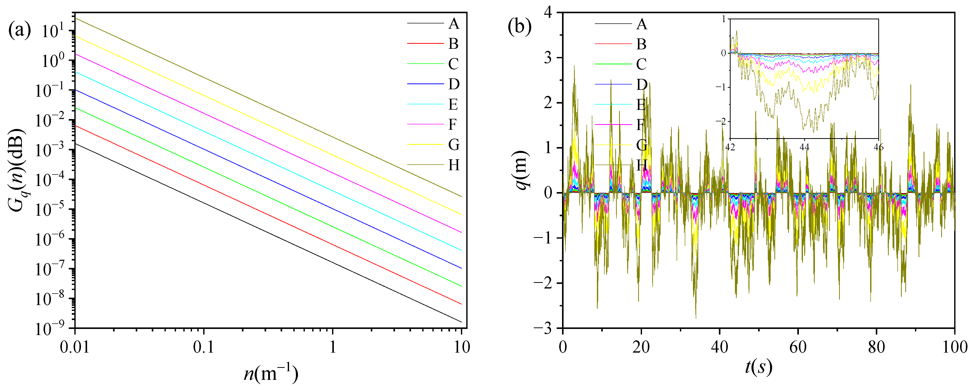
2.2. Mathematical Model of Road Excitation

2.2.1. Description of Road Excitation at Single Wheel

The pavement unevenness function is the variation q(I) in the height q of the road surface with respect to the reference level, along the length I of the road alignment, also known as the longitudinal profile of the pavement. Experimental tests have proved that the pavement unevenness can be modeled as a stationary and ergodic Gaussian random signal. The statistical characterization of pavement unevenness is mainly based on the self-power spectrum of the pavement (referred to as the power spectrum). The power spectral density is defined as the “power” (mean square value) in the unit frequency band. Therefore, the power spectral density at the spatial frequency is as follows [62]:

$$G_q\left(n\right)=\underset{\mathsf{\Delta }n\to 0}{\lim }\frac{{\sigma }_{q~\mathsf{\Delta }n}^2}{\mathsf{\Delta }n},$$

(18)

where ${\sigma }_{q~\mathsf{\Delta }n}^2$ is the “power” contained in the pavement power spectral density in the frequency band ∆n, and n is the number of waves per unit length. The vertical displacement self-power spectral density of pavement unevenness on longitudinal length I can be fitted using the following equation:

$$G_q\left(n\right)=G_q\left(n_0\right){\left(\frac{n}{n_0}\right)}^{-W},$$

(19)

where n is the spatial frequency (m⁻¹), indicating how many wavelengths are included in each meter length; n₀ is the reference spatial frequency, n₀ = 0.1 m⁻¹; G_q(n₀) is the power spectral density of the pavement at the reference spatial frequency, also known as the pavement unevenness coefficient; and W is the frequency index of the graded pavement spectrum. W is used to represent the frequency structure of the spectral density of the pavement, which is expressed as a function of the slope of the spectral density in double logarithmic coordinates. In the standard graded pavement spectrum, W is equal to 2.

Table 2. The 8-class classification of road surface unevenness.

Category	Gq(n0)/(10−6 m3) (n0 = 0.1 m−1)	σq/(10−3 m) (0.011 m−1 < n < 2.83 m−1)
A	16	3.81
B	64	7.61
C	256	15.23
D	1024	30.45
E	4096	60.90
F	16,384	121.89
G	65,536	243.61
H	262,144	487.22

shows the eight-class classification for describing pavement unevenness [63].

The spatial power spectral density G_q(n) describes the statistical characteristics of pavement unevenness in the length direction. The spatial frequency cannot be directly used for the calculation and analysis of vehicle vibration systems. What kind of uneven impact a vehicle encounters depends not only on the structural properties of the road surface, but also on the driving speed of the vehicle. When a vehicle travels on a given road surface at a certain speed, it will “collide” with these uneven points on the road surface at certain time intervals, resulting in a “time frequency”. When the spatial frequency n or bandwidth ∆n is constant, the temporal frequency f or bandwidth ∆f varies proportionally with the speed of the vehicle, which means that the following equation holds:

$$f=un.$$

(20)

At a certain speed, the resonance components of the vertical displacement of unevenness contained in the time–frequency bandwidth ∆f corresponding to the spatial frequency bandwidth ∆n are the same; therefore, its energy is still ${\sigma }_{q~\mathsf{\Delta }n}^2$. Therefore, the power spectral density of converting spatial frequency to temporal frequency can be expressed as follows [64]:

$$G_q\left(f\right)=\underset{\mathsf{\Delta }n\to 0}{\lim }\frac{{\sigma }_{q~\mathsf{\Delta }n}^2}{u\mathsf{\Delta }n}=\frac{G_q\left(n\right)}{u}=G_q\left(n_0\right)n_0^2\frac{u}{f^2}.$$

(21)

If the power spectral density is expressed in terms of angular frequency ω = 2πf, the above equation can be rewritten as follows:

$$G_q\left(\omega \right)={(2\pi )}^2{G}_q\left(n_0\right)n_0^2\frac{u}{{\omega }^2}.$$

(22)

However, in the above equation, G_q(ω)→∞ when ω→0, so it is not in line with the engineering reality. Therefore, it is necessary to set the lower cutoff frequency ω₀ = 2πun₀₀; then, the above equation is transformed into the following form:

$$G_q\left(\omega \right)={(2\pi )}^2{G}_q\left(n_0\right)n_0^2\frac{u}{{\omega }^2+{\omega }_0^2},$$

(23)

where n₀₀ = 0.01 m⁻¹ is the cutoff spatial frequency.

There are many methods to construct the time domain model of a pavement, mainly including the harmonic superposition method, random sequence generation method, inverse Fourier transform method, and filtered white noise method. The filtered white noise method can be directly employed to determine the pavement model parameters based on the pavement unevenness coefficient and driving speed. Let us assume that a linear system H(jω) adopts Gaussian white noise S(ω) with unit intensity of 1 as the system input and the pavement unevenness G_q(ω) as the system output. The frequency response function can be expressed as follows [65]:

$$H\left(j\omega \right)=\frac{a}{b+j\omega },$$

(24)

So, the power spectral density G_q(ω) of pavement unevenness is shown below:

$$G_q\left(\omega \right)=‖H(j\omega )‖S\left(\omega \right).$$

(25)

By reverse solving, we obtain the following:

$$\left\{\begin{array}{l}a=2\pi n_0\sqrt{G_q\left(n_0\right)u}\\ b=2\pi n_{00}u\end{array}\right..$$

(26)

The frequency response function of this linear system is rephrased as follows:

$$H\left(j\omega \right)=\frac{2\pi n_0\sqrt{G_q\left(n_0\right)u}}{2\pi n_{00}u+j\omega },$$

(27)

So, the differential equation corresponding to this linear system is as follows [66]:

$$\dot{q}(t)=-2\pi n_{00}uq(t)+2\pi n_0\sqrt{G_q\left(n_0\right)u}\cdot w(t),$$

(28)

where w(t) is the time domain signal for white noise and q(t) is the time domain signal for the pavement unevenness spectrum.

The signal variation diagram presented in Figure 2 illustrates the road excitation for the eight-class classification of road surface unevenness, showcasing two key representations: (a) the spatial frequency domain signal and (b) the time domain signal at a vehicle speed u = 60 km/h. This diagram serves as a crucial component in the study of road surface analysis and classification, particularly in the context of assessing road conditions for vehicular travel. Vehicles have four road excitations; therefore, the random road excitation model needs to consider the delay between the front and rear-wheel tracks and the coherence between the left and right-wheel tracks.

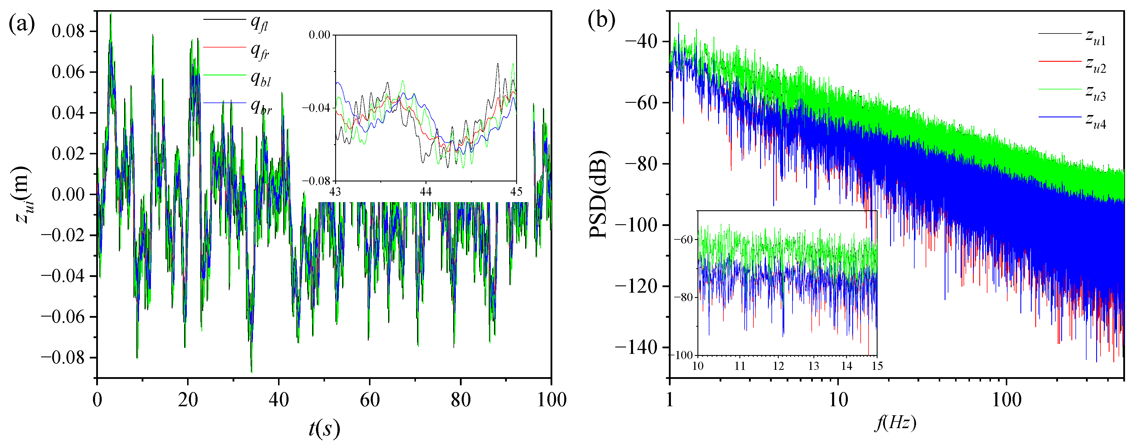
2.2.2. Delay between Front and Rear-Wheel Tracks

If the vehicle is traveling in a straight line at a constant speed, the time delay of the front and rear wheel pavement excitation on the same side is T = (l₁ + l₂)/u. The front and rear wheel pavement excitation has large pure time delay characteristics, and the continuous domain transfer function of the time delay model is e^Ts. The transfer function for the pure time delay model is more difficult to analyze directly because it is essentially an infinite dimensional system. The Pade approximation is a rational polynomial approximation, which tends to be more accurate than the truncated Taylor’s approximation. The higher the order of the Pade approximation, the higher the accuracy, but the more complicated the expression. The first-order Pade approximation is used to approximate the pure delay model [67]:

$$e^{Ts}\approx \left(1-\frac{Ts}{2}\right)/\left(1+\frac{Ts}{2}\right).$$

(29)

where s is the Laplace operator. Therefore, the relationship between the front and rear wheel excitation inputs satisfies the following:

$${\dot{q}}_b=-\frac{2}{T}{q}_b-{\dot{q}}_f+\frac{2}{T}{q}_f,$$

(30)

where q_f(I) and q_b(I) are the statistical characteristics of the front and rear-wheel tracks. The time domain models for the road excitation of the front and rear wheels are expressed as follows:

$$\left(\begin{array}{c}{\dot{q}}_f\\ {\dot{q}}_b\end{array}\right)=\left(\begin{array}{cc}-2\pi n_{00}u& 0\\ 2\pi n_{00}u+\frac{2}{T}& -\frac{2}{T}\end{array}\right)\left(\begin{array}{c}{q}_f\\ q_b\end{array}\right)+\left(\begin{array}{c}2\pi n_0\sqrt{G_q\left(n_0\right)u}\\ -2\pi n_0\sqrt{G_q\left(n_0\right)u}\end{array}\right)w(t).$$

(31)

where w(t) is the white noise.

2.2.3. Coherence between Left and Right-Wheel Tracks

The phase spectrum of the left and right-wheel tracks is equal to φ_ll(n) = 0, which means that the statistical characteristics of the left and right-wheel tracks q_l(I) and q_r(I) are the same, that is, the self-power spectrum of the left and right-wheel tracks is the same, meaning G_ll(n) = G_rr(n) = G_q(n), where G_ll(n) and G_rr(n) are the self-power spectrum of the left and right-wheel tracks, respectively. The random process of the unevenness of the left and right tracks on the same road has a cross-spectrum, that is, the two tracks are coherent. Therefore, the spatial coherence must be taken into account in describing the time domain model of the two road excitations. The cross-spectrum between the left and right-wheel tracks can be represented as follows:

$$G_{lr}\left(n\right)=‖G_{lr}\left(n\right)‖{\mathrm{e}}^{-\mathrm{j}{\varphi }_{lr}\left(n\right)},$$

(32)

where $‖G_{lr}\left(n\right)‖$ can be determined by the correlation function of the left and right-wheel tracks [68]:

$${\mathrm{coh}}_{lr}^2\left(n\right)=\frac{{‖G_{lr}\left(n\right)‖}^2}{G_{ll}\left(n\right)G_{rr}\left(n\right)}=\frac{{‖G_{lr}\left(n\right)‖}^2}{G_q\left(n\right)G_q\left(n\right)}.$$

(33)

Therefore, the following relationship G_lr(n) = coh_lr(n)·G_q(n) can be obtained.

Considering the coherence of the left and right wheels, the white noise w_r(t) at the right wheel track can be simulated by the combination of the white noise w_l(t) at the left-wheel track and another incoherent unit of white noise w_z(t). The above description indicates that the following equation is valid:

$$w_r\left(\omega \right)=H_{r-l}\left(\omega \right)w_l\left(\omega \right)+H_{r-\mathrm{z}}\left(\omega \right)w_z\left(\omega \right).$$

(34)

where H_r-l is the transfer function corresponding to the white noise w_l(t), and H_r-z is the transfer function corresponding to the white noise w_z(t). The self-spectral functions of the left and right-wheel tracks are equal, indicating that ‖H_r-l‖² + ‖H_r-z‖² = 1. According to the theory of random vibration, the frequency response function H_r-l of the input system w_l(t) satisfies the following equation:

$$H_{r-l}\left(\omega \right)=\frac{G_{lr}(\omega )}{G_{ll}(\omega )}={\mathrm{coh}}_{lr}\left(\omega \right).$$

(35)

The widely used empirical formula for the coherence function is coh_lr(ω) = e^{−ρ(l3 + l4)ω/πu}. For the convenience of simulation, the amplitude frequency characteristics are optimized by approximating the transfer function H_r-l of the left and right-wheel tracks to a second-order transfer function. At the same time, we also transform H_r-z into second-order transfer function form. The above indicates that the following equation can be obtained:

$$\left\{\begin{array}{c}{H}_{r-l}\left(j\omega \right)=\frac{a_0+a_{1}j\omega +a_2{\left(j\omega \right)}^2}{b_0+b_{1}j\omega +b_2{\left(j\omega \right)}^2}\\ H_{r-z}\left(j\omega \right)=\frac{c_0+c_{1}j\omega +c_2{\left(j\omega \right)}^2}{b_0+b_{1}j\omega +b_2{\left(j\omega \right)}^2}\end{array}\right.,$$

(36)

where a₀ = 1.000, a₁ = 0.0736k, a₂ = 0.0239k², b₀ = 1.0696, b₁ = 2.8390k, b₂ = 0.8330k², c₀ = 0.3795, c₁ = 2.6367k, c₂ = 0.8327k², and k = ρ(l₁ + l₂)/πu [69]. By introducing the intermediate state variables ξ(t) = [ξ₁(t), ξ₂(t)]^T and Ψ(t) = [Ψ₁(t), Ψ₂(t)]^T, the above equation can be decomposed into the following two state equations:

$$\left\{\begin{array}{c}\left(\begin{array}{c}{\dot{\xi }}_1(t)\\ {\dot{\xi }}_2(t)\end{array}\right)=\left(\begin{array}{cc}-\frac{b_1}{b_2}& -\frac{b_0}{b_2}\\ 1& 0\end{array}\right)\left(\begin{array}{c}{\xi }_1(t)\\ {\xi }_2(t)\end{array}\right)+\left(\begin{array}{c}\frac{1}{b_2}\\ 0\end{array}\right)w_l\left(t\right)\\ \left(\begin{array}{c}{\dot{\Psi }}_1(t)\\ {\dot{\Psi }}_2(t)\end{array}\right)=\left(\begin{array}{cc}-\frac{b_1}{b_2}& -\frac{b_0}{b_2}\\ 1& 0\end{array}\right)\left(\begin{array}{c}{\Psi }_1(t)\\ {\Psi }_2(t)\end{array}\right)+\left(\begin{array}{c}\frac{1}{b_2}\\ 0\end{array}\right)w_z\left(t\right)\end{array}\right.,$$

(37)

The time domain expression for the white noise at the right-wheel track is as follows:

$$\begin{array}{ll}{w}_r\left(t\right)& =\left(\begin{array}{cc}{a}_1-\frac{a_2{b}_1}{b_2}& a_0-\frac{a_2{b}_0}{b_2}\end{array}\right)\left(\begin{array}{c}{\xi }_1(t)\\ {\xi }_2(t)\end{array}\right)+\frac{a_2}{b_2}{w}_l\left(t\right)\\ & +\left(\begin{array}{cc}{c}_1-\frac{c_2{b}_1}{b_2}& c_0-\frac{c_2{b}_0}{b_2}\end{array}\right)\left(\begin{array}{c}{\Psi }_1(t)\\ {\Psi }_2(t)\end{array}\right)+\frac{c_2}{b_2}{w}_z\left(t\right).\end{array}$$

(38)

The right track stochastic process is derived from the known left track stochastic process by establishing a coherent relationship between the left and right wheels. When establishing a road model, w_l(t) can first generate the left-wheel track, and through the intermediate state variables ξ(t) = [ξ₁(t), ξ₂(t)]^T and Ψ(t) = [Ψ₁(t), Ψ₂(t)]^T, the time domain model of the white noise input w_r(t) at the right wheel can be obtained. The time domain models for the road excitation of the left and right wheels are expressed as follows:

$$\left\{\begin{array}{l}{\dot{q}}_l(t)=-2\pi n_{00}uq(t)+2\pi n_0\sqrt{G_q\left(n_0\right)u}\cdot w_l(t)\\ {\dot{q}}_r(t)=-2\pi n_{00}uq(t)+2\pi n_0\sqrt{G_q\left(n_0\right)u}\cdot w_r(t)\end{array}\right..$$

(39)

Figure 3 depicts the variation in road excitation at C-class pavement unevenness for a vehicle speed of 60 km/h. Figure 3a illustrates the time domain signal, while Figure 3b showcases the time–frequency domain signal. This analysis offers a comprehensive understanding of the pavement’s response to varying speeds.

3. Methods

3.1. Fractional-Order PI^λD^μ

3.1.1. Fractional-Order Calculus Theory

Fractional calculus is an extension of integer calculus. When the order of differentiation and integration is fractional, integer calculus becomes fractional calculus. Three definitions of fractional-order calculus that have been used in the control field include the Grunwald–Letnikov formulation, the Riemann–Liouville formulation, and the Caputo formulation [70].

The Grunwald–Letnikov formulation is based on the definition of higher-order derivatives of classical integer orders, and is derived through induction to generalize the orders and factorials of integer-order calculus to non-integer orders. The Grunwald–Letnikov formulation for the α-th derivative of function f(t) is expressed as follows [71]:

$${ }_{t_0}^{GL}{D}_t^{\alpha }f\left(t\right)=\underset{h\to 0}{\lim }\frac{1}{h^{\alpha }}{\displaystyle \sum }_{j=0}^{\left[\left(t-t_0\right)/h\right]}{(-1)}^j\left(\begin{array}{l}\alpha \hfill \\ j\hfill \end{array}\right)f\left(t-jh\right),t>0,\alpha \in R^{+},$$

(40)

where [·] is the round operator, t₀ is the lower limit, t is the upper limit, α is the order, and

$$\left(\begin{array}{l}\alpha \hfill \\ j\hfill \end{array}\right)=\frac{\alpha \left(\alpha +1\right)\cdots \left(\alpha +j-1\right)}{j!}=\frac{\alpha !}{j!\left(\alpha -j\right)!}.$$

(41)

Equation (40) corresponds to fractional-order differentiation and fractional-order integration for α > 0 and α < 0, respectively, while for α = 0, it corresponds to the primitive function f(t).

The Riemann–Liouville formulation needs to solve an initial value problem that is theoretically achievable but lacks physical meaning in reality, and thus is limited in its application. The Riemann–Liouville formulation for fractional integration is defined as follows [72]:

$${}_{t_0}{}^{RL}D_t^{-\alpha }f(t)=\frac{1}{\mathsf{\Gamma }(\alpha )}{\displaystyle {\int }_{t_0}^t\frac{f(\tau )}{{(t-\tau )}^{1-\alpha }}}d\tau ,$$

(42)

where Γ(α) is the gamma function. In the Riemann–Liouville formulation, the definition of fractional differentiation depends on fractional integration. The Riemann–Liouville formulation for fractional differentiation is defined as follows:

$${ }_{t_0}^{RL}{D}_t^{\alpha }f\left(t\right)=\frac{1}{\mathsf{\Gamma }\left(n-\alpha \right)}\frac{d^n}{d{t}^n}{{\displaystyle \int }}_{t_0}^t\frac{f\left(\tau \right)}{{(t-\tau )}^{\alpha -n+1}}d\tau ,$$

(43)

where n − 1 < α ≤ n, and n = [α].

The Caputo formulation is a commonly used method for describing systems of fractional order and can deal with initial condition problems for systems of fractional order. The fractional-order differentiation of the Caputo formulation is defined as follows [73]:

$${ }_{t_0}^C{D}_t^{\alpha }f\left(t\right)=\frac{1}{\mathsf{\Gamma }\left(m-\alpha \right)}{{\displaystyle \int }}_{t_0}^t\frac{f^{\left(m\right)}\left(\tau \right)}{{(t-\tau )}^{1+\alpha -m}}d\tau ,$$

(44)

where m = [α]. Fractional integration for the Caputo formulation is defined as follows:

$${ }_{t_0}^C{D}_t^{-\alpha }f\left(t\right)=\frac{1}{\mathsf{\Gamma }\left(\gamma \right)}{{\displaystyle \int }}_{t_0}^t\frac{f\left(\tau \right)}{{(t-\tau )}^{1-\alpha }}d\tau .$$

(45)

Fractional-order PID modeling is based on Grünwald–Letnikov fractional-order calculus for numerical computation in the time domain.

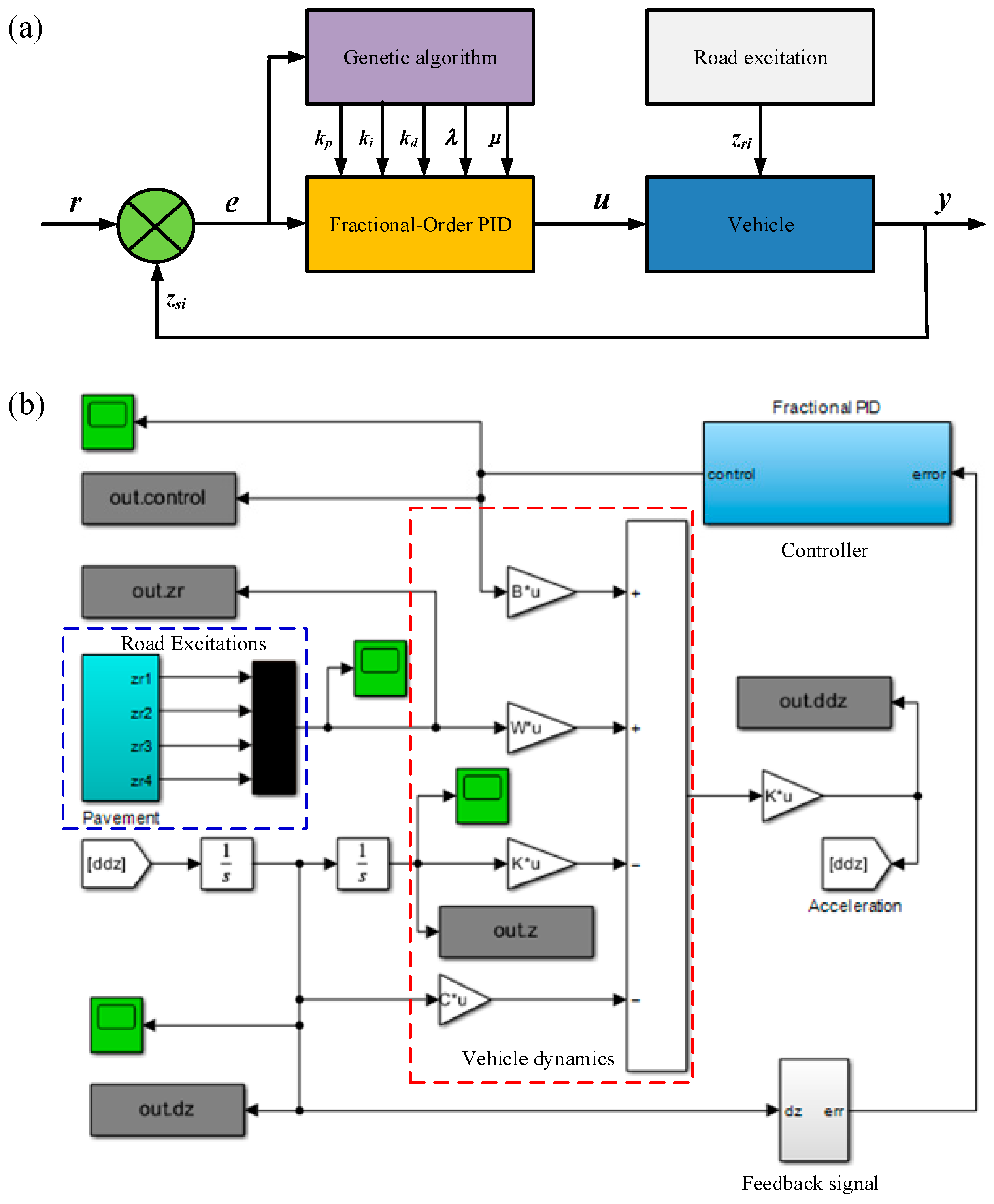
3.1.2. Structure of Fractional-Order PI^λD^μ Controller

The classical PID controller is simple in principle and has strong robustness and adaptability. The classical PID controller consists of proportional part P, integral part I, and differential part D. The classical PID control algorithm is shown below [74]:

$$u(t)=k_{p}e(t)+k_i{\displaystyle \int e(t)dt+k_d\frac{de(t)}{dt}},$$

(46)

where k_p is the proportional amplification coefficient, k_i is the integral coefficient, k_d is the differential coefficient, u(t) is the control output, and e(t) is the deviation value of the system output.

The advantage of fractional-order calculus over integer-order calculus is that it can more accurately describe complex processes that are specific and complex with time spans and spatial autocorrelation. The fractional-order PID controller introduces the theory of fractional calculus on the basis of classical PID controllers, and its control algorithm can be expressed as follows:

$$u(t)=k_{p}e(t)+k_{i{t}_0}^{GL}{D}_t^{-\lambda }e(t)+k_{d{t}_0}^{GL}{D}_t^{\mu }e(t),$$

(47)

where λ and μ represent the order of integration and differentiation, respectively, 0 < λ, and μ < 1.

In the active suspension PID controller, the vibration speed deviation at the human–seat system is $e_c=0-{\dot{z}}_c$, and the active control force at the human–seat system is u_c. The suspension vibration speed deviation at the left front is $e_1=0-{\dot{z}}_{s1}$, and the active control force of the suspension at the left front is u₁. The suspension vibration speed deviation at the right front is $e_2=0-{\dot{z}}_{s2}$, and the active control force of the suspension at the right front is u₂. The vibration speed deviation at the left rear is $e_3=0-{\dot{z}}_{s3}$, and the suspension active control force at the left rear is u₃. The suspension vibration speed deviation at the right rear is $e_4=0-{\dot{z}}_{s4}$, and the suspension active control force at the left rear is u₄. Specifically, the controller input U is as follows:

$$U=\left(\begin{array}{c}{u}_c(t)=k_p{e}_c(t)+k_{i{t}_0}^{GL}{D}_t^{-\lambda }{e}_c(t)+k_{d{t}_0}^{GL}{D}_t^{\mu }{e}_c(t),\\ u_1(t)=k_p{e}_1(t)+k_{i{t}_0}^{GL}{D}_t^{-\lambda }{e}_1(t)+k_{d{t}_0}^{GL}{D}_t^{\mu }{e}_1(t),\\ u_2(t)=k_p{e}_2(t)+k_{i{t}_0}^{GL}{D}_t^{-\lambda }{e}_2(t)+k_{d{t}_0}^{GL}{D}_t^{\mu }{e}_2(t),\\ u_3(t)=k_p{e}_3(t)+k_{i{t}_0}^{GL}{D}_t^{-\lambda }{e}_3(t)+k_{d{t}_0}^{GL}{D}_t^{\mu }{e}_3(t),\\ u_4(t)=k_p{e}_4(t)+k_{i{t}_0}^{GL}{D}_t^{-\lambda }{e}_4(t)+k_{d{t}_0}^{GL}{D}_t^{\mu }{e}_4(t),\end{array}\right..$$

(48)

The fractional-order PID controller has time memory, meaning that the output of the controller depends not only on the current control error, but also on the history of previous control errors. This time memory allows the fractional-order PID controller to better adapt to the dynamic characteristics of the system.

Professor Tepljakov and his team [75] have developed a software for calculating fractional calculus called FOMCON (readers can access this website at https://fomcon.net; accessed on 25 January 2024). This software has the capability to perform complex mathematical operations related to fractional calculus, making it a valuable tool for researchers and practitioners in the field. The software has been well received in the scientific community and has been published in several high-impact journals. Its user-friendly interface and accurate results make it a valuable asset for anyone working with fractional calculus. FOMCON has the potential to revolutionize the way we approach and solve mathematical problems related to fractional calculus, and its impact on the field is expected to grow in the coming years. The latest update of FOMCON introduces a new feature to its Fractional-Order Differential Equation (FODE) solver, based on the Grünwald–Letnikov method. In addition to the default first-order solver, users now have the option to choose higher-order numerical solvers, including second and third-order formats, for computing the time domain response of systems described by fractional-order transfer function objects. This enhancement provides users with increased flexibility and precision in their simulations, allowing for more accurate and detailed analysis of complex systems. Readers can also consult the Supplementary Materials for further details and information.

3.2. Genetic Algorithm

3.2.1. Process of Genetic Algorithm

The control effect of a PID controller depends on the combination of the proportional amplification coefficient k_p, integral coefficient k_i, and differential coefficient k_d. Traditional methods often use the trial-and-error method. The trial-and-error method is optimized in the order of proportion, integration, and differentiation. After each coefficient setting, the system’s operation should be observed, and then each coefficient value should be adjusted according to the system’s operation until the optimal control effect is achieved. In general, the response speed of the system will increase with the increase in the proportional coefficient, which is beneficial for reducing static errors. However, the proportional coefficient that exceeds the range will generally cause the system to have significant overshoot and also worsen oscillation stability. Reducing the integral coefficient is beneficial for reducing overshoot and making the system stable, but it slows down the speed of eliminating static errors. Increasing the differential coefficient is beneficial for accelerating the system’s response and reducing overshoot, and also weakens its resistance to interference. It can be seen that the parameter adjustment of the trial-and-error method is difficult, and the performance of the PID algorithm highly depends on the selection of parameters. For complex systems, multiple experiments and adjustments are often required to achieve good control results [76].

The genetic algorithm is a method of searching for optimal solutions by simulating natural evolution processes. The parameters of the PID controller can be self-tuned through genetic algorithms. Self-tuning is the process of adjusting controller parameters through program optimization, without the need for the trial-and-error method. The genetic algorithm is an optimization algorithm based on natural selection and genetic evolution theory, which simulates the evolution process of biological populations and gradually optimizes the fitness of the population through gene combination, mutation, crossover, and other operations, ultimately obtaining the optimal solution, as shown in Figure 4 [77].

3.2.2. Implementation of Genetic Algorithm

The following specific process introduces the actual process of genetic algorithm optimization. Firstly, the seat vertical vibration acceleration, body vertical vibration acceleration, pitch angle acceleration, roll angle acceleration, suspension dynamic deflection at four tires, and tire dynamic displacement are selected as performance indicators. Then, they are divided by the passive suspension performance indicators under the same operating conditions to construct the fitness function f(k) of the genetic algorithm [78]:

$$\left(\begin{array}{l}\min f(k)=\frac{AV{B}_1(k)}{AV{B}_1^{pas}}+\frac{AV{B}_2(k)}{AV{B}_2^{pas}}+\frac{AV{B}_3(k)}{AV{B}_3^{pas}}+\frac{AV{B}_3(k)}{AV{B}_4^{pas}}+{\displaystyle \sum _{i=1}^4\frac{SW{S}_i(k)}{SW{S}_i^{pas}}+{\displaystyle \sum _{i=1}^4\frac{DT{D}_i(k)}{DT{D}_i^{pas}}}}\\ k=(k_p,k_i,k_d,\lambda ,\mu ),0\le k_p,k_i\le 2^{14}-1,0\le k_d\le 2^7,0\le \lambda \le 1,0\le \mu \le 1\end{array}\right.,$$

(49)

where AVB₁(k), AVB₂(k), AVB₃(k), and AVB₄(k) represent the root mean square values of seat vertical vibration, body vertical vibration acceleration, pitch angle acceleration, and roll angle acceleration, respectively. SWS_i(k) represents the root mean square value of suspension dynamic deflection, and DTD_i(k) represents the root mean square value of tire dynamic displacement. AVB_i^pas, SWS_i^pas, and DTD_i^pas are the root mean square values of the corresponding performance indicators of passive suspension under the same operating conditions as the active suspension system. It should be noted that the performance indicators of active suspension should be superior to those of passive suspension, that is to say, the following limiting conditions should be met:

$$\left\{\begin{array}{l}AV{B}_i(k)\le AV{B}_i^{pas}\\ SW{S}_i(k)\le SW{S}_i^{pas}\\ DT{D}_i(k)\le DT{D}_i^{pas}\end{array}\right..$$

(50)

To limit the solution, we adopt the idea of penalty functions. That is to say, if the root mean square value of a performance indicator of the active suspension is detected to be greater than the root mean square value of a performance indicator of the passive suspension, then its fitness function is increased as a penalty, so that the chromosome of this individual is not considered a genetic object as much as possible. The specific expression is as follows:

$$\left(\begin{array}{l}f(k)=\frac{AV{B}_1(k)}{AV{B}_1^{pas}}+\frac{AV{B}_2(k)}{AV{B}_2^{pas}}+\frac{AV{B}_3(k)}{AV{B}_3^{pas}}+\frac{AV{B}_3(k)}{AV{B}_4^{pas}}+{\displaystyle \sum _{i=1}^4\frac{SW{S}_i(k)}{SW{S}_i^{pas}}+{\displaystyle \sum _{i=1}^4\frac{DT{D}_i(k)}{DT{D}_i^{pas}}}}+N(k)\\ if AV{B}_i(k)\ge AV{B}_i^{pas} \mathrm{or} SW{S}_i(k)\ge SW{S}_i^{pas} \mathrm{or} DT{D}_i(k)\ge DT{D}_i^{pas}\end{array}\right.,$$

(51)

where N(k) is the penalty degree, and N(k) has the following expression form:

$$\left\{\begin{array}{l}N(k)={\displaystyle \sum _{j=1}^{N_{total}}{R}_j{f}_j^{\beta }(k),if f_j(k)\ge 1}\\ f_j(k)\in [AV{B}_i(k)/AV{B}_i^{pas},SW{S}_i(k)/SW{S}_i^{pas},DT{D}_i(k)/DT{D}_i^{pas}]\end{array}\right.,$$

(52)

where β = 2 is the parameter and N_total is the total number of active suspension performance indicators. R_j is the penalty factor:

$$R_j=\left\{\begin{array}{l}1.0, if f_j(k)\ge 1 \mathrm{and} f_j(k)\in AV{B}_i(k)/AV{B}_i^{pas}\\ 0.5,if f_j(k)\ge 1 \mathrm{and} f_j(k)\in SW{S}_i(k)/SW{S}_i^{pas}\\ 0.1,if f_j(k)\ge 1 \mathrm{and} f_j(k)\in DT{D}_i(k)/DT{D}_i^{pas}\end{array}\right.,$$

(53)

The penalty varies with the number of iterations, indicating that this is a dynamic penalty process.

Encoding refers to converting a given real number into a binary string. The length of a binary string depends on the accuracy requirements. Here, the chromosome consists of five segments, corresponding to k_p, k_i, k_d, λ, and μ. Assuming that a chromosome segment k_j can be represented by a 14-bit unsigned binary number, the encoding corresponding to the chromosome segment k_j is b₁₂b₁₁b₁₀…b_i…b₃b₂b₁. The corresponding decoding formula is as follows [79]:

$$K_i=U_{min}+({\displaystyle \sum _{j=1}^{12}{b}_j\cdot 2^{j-1}})\cdot \frac{U_{max}-U_{min}}{2^{12}-1},$$

(54)

where U_min and U_max are the range of values for phenotype K_i, respectively, that is, K_i∈[U_min, U_max]. Thus, a 60-bit unsigned binary number formed by connecting all chromosome segments together forms the genotype K of the individual, which represents a feasible solution. For example, the phenotype corresponding to genotype K = 000000000001000000000001000000000001000000000001000000000001 is k = (1.0, 1.0, (2⁶ − 1)/(2¹² − 1), 1/(2¹² − 1), 1/(2¹² − 1)), which means k_p = 1.0, k_i = 1.0, k_d = (2⁶ − 1)/(2¹² − 1), λ = 1/(2¹² − 1), and μ = 1/(2¹² − 1). The phenotype k and genotype K of an individual can be converted into each other through encoding and decoding programs.

The initial population is the initial population data P₀ that represent the starting search point for the genetic algorithm to perform evolutionary operations on the population. The size of the population is taken as N, where N = 100, which means that the population is composed of 100 individuals. Each individual’s genotype can be randomly generated. In genetic algorithms, the fitness of each individual is used to evaluate their level of superiority and inferiority, thereby determining their genetic opportunities. After converting an individual’s genotype to phenotype, the minimum value of the fitness function f(k) can be used as the optimization objective, so the objective function value can be directly used as the individual’s fitness.

The selection operation inherits individuals with greater fitness from the current population into the next-generation population according to a certain rule or model. Individuals with greater fitness are generally required to have more opportunities to be inherited into the next-generation population. A probability proportional to fitness is used to determine the number of individual replications into the next generation of the population. The roulette-wheel approach is chosen for the selection operation, that is, the sum of the fitness of all individuals in the population is first calculated as follows:

$$FI={\displaystyle \sum _{i=1}^N\begin{array}{cc}{f}_i(k),& i=1,\cdots ,N,\end{array}}$$

(55)

Second, the magnitude of the relative fitness of each individual is calculated as the probability that each individual will be inherited into the next generation of the population:

$$\begin{array}{cc}{P}_i=f_i(k)/FI,& i=1,\cdots ,N\end{array},$$

(56)

Then, the cumulative probability of each chromosome is calculated as follows:

$$Q_i={\displaystyle \sum _{j=1}^i{P}_j}, i=1,\cdots ,N.$$

(57)

Each cumulative probability value forms a region and the last chromosome satisfies Q_N = 1. Finally, N random numbers r between 0 and 1 are generated, and based on this random number, the number of times each individual is selected is determined. If Q_l−1 ≤ r ≤ Q_l, the l-th chromosome is selected.

The cross-over operation is the main process of generating new individuals in genetic algorithms, which exchanges some chromosomes between two individuals with a certain probability. A single-point crossover method is used, in which the populations are first randomly paired, followed by the randomization of crossover positions, and finally by mutual exchange of some genes between the paired chromosomes. The crossover operation probability P_jc = 70% is chosen, which determines that there is a 70% probability that an individual chromosome of the parent will be crossed over in the crossover operation at the statistical level. If the crossover probability is too large, it may lead to too much mixing of individual genetic information, making the search process too random, thus affecting the performance of the algorithm. If the crossover probability is too small, it may lead to too little individual gene information, making the search process too limited, thus affecting the convergence speed of the algorithm.

The mutation operation is a method of generating new individuals by changing the gene value of one bit or some bits of an individual with a small probability. Mutation operations are performed using the basic bit mutation method, in which the location of the gene mutation is first determined for each individual, and then the value of the original gene at the mutation point is reversed according to a certain probability. The probability of mutation is assumed to be P_by = 0.01%, which determines that there is a 0.01% probability that an individual chromosome of the parent generation will be mutated in the mutation operation at the statistical level. This algorithm has a total of 6000 gene bits, which represents 60 bits per generation that undergo mutation operations in a statistical sense.

A new generation of population P(t + 1) can be obtained after a round of selection, crossover, and mutation operations on population P(t). The reproduction number (maximum number of iterations) is taken as T_max = 100. The population will reach the global optimum in terms of fitness after generations of evolution.

The Genetic Algorithm Toolbox for MATLAB (version R2022b) was developed by the Department of Automatic Control and Systems Engineering at The University of Sheffield, UK [80]. The purpose of this development was to provide control engineers with access to genetic algorithms within the existing framework of a computer-aided control system design package. This toolbox aims to make genetic algorithms more accessible and applicable to the field of control engineering (readers can access this website at http://uos-codem.github.io/GA-Toolbox; accessed on 25 January 2024). Readers can also refer to the Supplementary Materials for additional information.

4. Results

The 8-DoF vehicle model is a complex dynamic system, and controlling it requires efficient algorithms to optimize controller parameters. In this case, using a genetic algorithm to optimize the fractional-order PID controller is an effective method (please refer to Supplementary Material Procedure).

First, we need to define the parameter space of the fractional-order PID controller, including the proportional coefficient, integral coefficient, derivative coefficient, and fractional-order parameters. Next, we can use a genetic algorithm to search this parameter space to find the optimal controller parameters. By simulating the process of natural selection, crossover, and mutation, genetic algorithms can search for better solutions in the parameter space. Through this process, genetic algorithms can search for optimal fractional-order PID controller parameters in the parameter space, thereby achieving efficient control of the 8-degree-of-freedom vehicle model, enabling it to exhibit good dynamic characteristics and robustness under various operating conditions, as shown in Figure 5a.

As shown in Figure 5b, modeling the vibration dynamics of a vehicle in Simulink and simulating the smoothness evaluation index can be achieved by the following steps. First, Simulink is used to construct the differential equations of the car vibration dynamics, including the suspension system, tires, body, and other components of the vehicle. Then, for the control problem of the vehicle vibration model, the control system toolbox in Simulink can be used to optimize the fractional-order PID controller using the genetic algorithm. The mathematical model of the fractional-order PID controller needs to be established and integrated into the vehicle vibration model. Using the optimization toolbox in Simulink, the objective function and constraints of the genetic algorithm optimization, as well as the parameter ranges of the fractional-order PID controller, can be set to optimize the controller parameters. This ensures that the vehicle has good vibration suppression performance under different road excitations. Finally, in order to evaluate the smoothness of the vehicle, the measurement module of the smoothness evaluation indexes, such as acceleration sensors, can be added in Simulink. By simulating the vibration response of the vehicle under different road excitations and combining the smoothness evaluation indexes, the smoothness performance of the vehicle can be comprehensively evaluated.

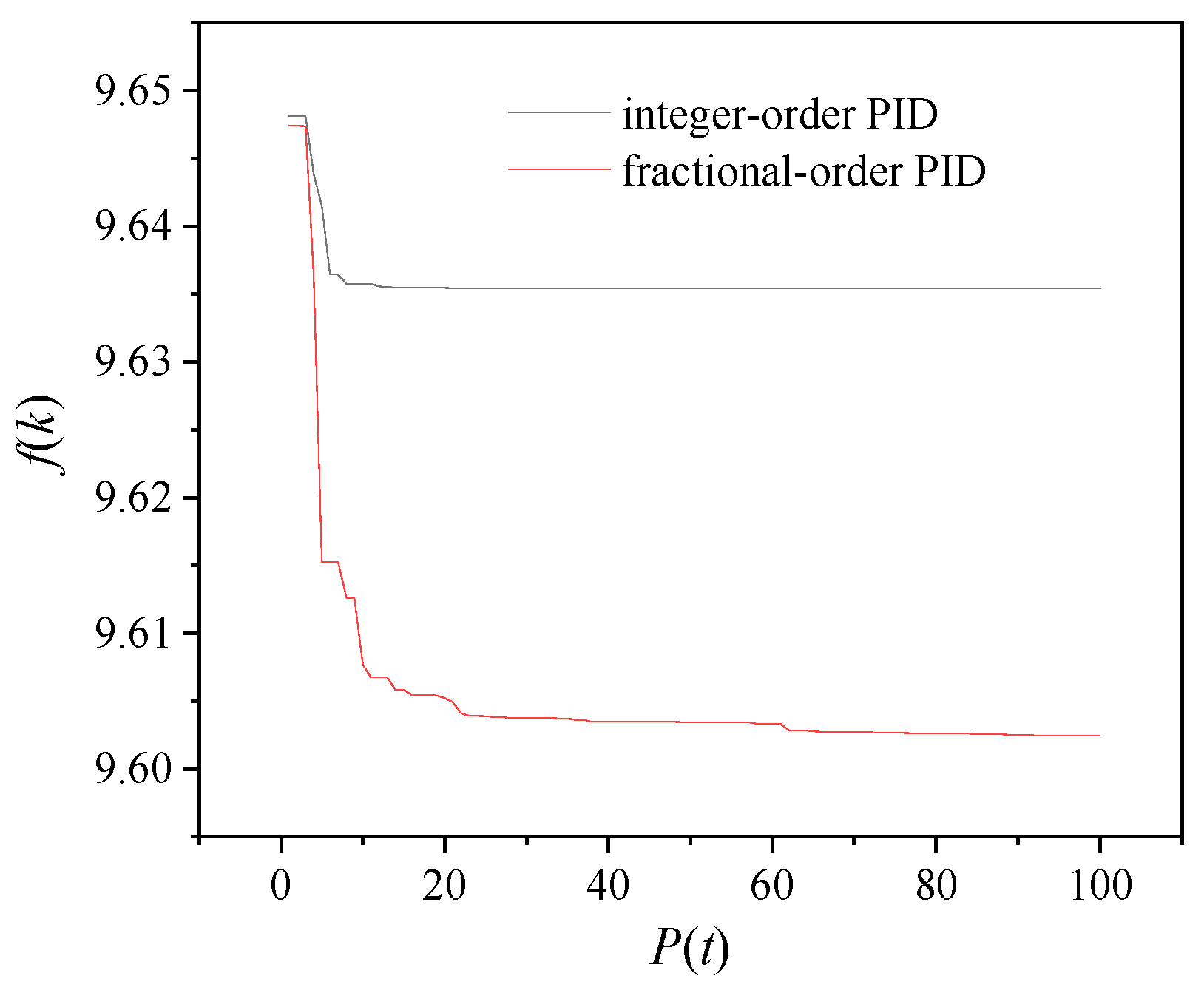
4.1. Variations in Fitness Function

As shown in Figure 6, the fitness functions f(k) of both fractional-order PID and integer-order PID control decrease with the increase in genetic generations. This is because as the genetic generations increase, the individuals in the population gradually converge, and individuals with less fitness are gradually eliminated, while individuals with greater fitness are preserved and reproduced. Therefore, overall fitness functions show a decreasing trend. In addition, the fitness function of the fractional-order PID control is smaller than that of the integer-order PID control. This is because fractional-order PID control has more flexible control characteristics compared to integer-order PID control, and can better adapt to complex control systems. Therefore, the performance of the fractional-order PID controller in terms of fitness function will be superior, and its fitness function will be relatively smaller.

Figure 7a shows the variation in the integer-order PID control parameters [k_p, k_i, and k_d], while Figure 7b shows the variation in the fractional-order PID control parameters [k_p, k_i, k_d, λ, and μ]. The trend of PID control parameters [k_p, k_i, k_d, λ, and μ] in the genetic algorithm is not monotonically increasing or decreasing but fluctuates during the iteration process. This is because the selection, crossover, and mutation operations in the genetic algorithm will generate new individuals, leading to changes in the values of the PID control parameters. During the iteration process of the genetic algorithm, the values of the PID control parameters [k_p, k_i, k_d, λ, and μ] will gradually converge to the vicinity of the optimal solution. Therefore, as the genetic generations increase, the trend of the PID control parameters will gradually decrease until it stabilizes around the optimal solution.

Table 3. Optimized PID parameter values.

PID	Integer-Order PID			Fractional-Order PID
	kp	ki	kd	kp	ki	kd	λ	μ
Value	2249.54424	2722.04638	0.30244	1059.56885	2777.72145	5.05887	0.47772	0.44056

displays the optimized PID parameter values for both integer-order and fractional-order PID controllers. For the integer-order PID controller, the proportional gain (k_p) is 2249.54424, the integral gain (k_i) is 2722.04638, and the derivative gain (k_d) is 0.30244. On the other hand, the fractional-order PID controller has a proportional gain (k_p) of 1059.56885, an integral gain (k_i) of 2777.72145, and a derivative gain (k_d) of 5.05887. Additionally, the fractional-order PID controller includes two additional parameters, λ and μ, with values of 0.47772 and 0.44056, respectively. These parameter values have been carefully optimized to achieve the desired control performance for the system under consideration.

4.2. Vibration Characteristics under C-Class Road

4.2.1. Changes in Control Signals

Figure 8 shows the time variations of control signals in a comparison of passive, integer-order PID, and fractional-order PID controllers. The control signal of the fractional-order PID controller exhibits more complex characteristics over time. As the fractional-order PID controller introduces the concept of fractional calculus, its control signal variation process may exhibit nonlinearity, singularity, and even chaotic behavior. In the context of a vehicle suspension system, the control signal variation of the fractional-order PID controller may demonstrate a faster response, but it may also be accompanied by larger fluctuations, especially when the system is initially disturbed by vibrations. Over time, the control signal of the fractional-order PID controller may gradually stabilize, but its variation process may still exhibit some degree of fluctuation and uncertainty.

Table 4. Statistical values of control signals.

PID		uc	u1	u2	u3	u4
Integer-order	RMS	129.32691	158.85456	121.82032	162.11136	166.07410
	AVE	10.86735	11.196190	10.941795	11.377870	11.12347
Fractional-order	RMS	126.30237	150.73555	118.37600	154.02911	161.77400
	AVE	8.87194	8.99648	8.85489	8.80790	8.66631

lists the root mean square (RMS) and average (AVE) values of control signals for integer-order PID control and fractional-order PID control. The formula for calculating the root mean square value is RMS = (x₁² + x₂² + … + x_n²)/n)/^1/2, where x₁, x₂, …, x_n are the individual values in the dataset, and n is the number of values in the dataset. The formula for calculating the mean is AVE = (x₁ + x₂ + … + x_n)/n. Firstly, the RMS values of the control signals for integer-order PID control are 129.32691, 158.85456, 121.82032, 162.11136, and 166.07410, while the RMS values for fractional-order PID control are 126.30237, 150.73555, 118.37600, 154.02911, and 161.77400. A comparison shows that the RMS values of the control signals for integer-order PID control are generally higher than those for fractional-order PID control, indicating that in these cases, the overall fluctuation of the integer-order systems is greater. Secondly, there are also differences in the AVE values of the control signals for integer-order and fractional-order PID control. The AVE values for integer-order PID control are 10.86735, 11.196190, 10.941795, 11.377870, and 11.12347, while the AVE values for fractional-order PID control are 8.87194, 8.99648, 8.85489, 8.80790, and 8.66631. The average value of the integer-order systems is larger, i.e., the overall deviation of data from the average value is greater for integer-order systems. Thus, the fluctuation in and deviation of data from the average value are both relatively greater for integer-order systems, while they are relatively smaller for fractional-order systems.

4.2.2. Variations in Performance Indicators in the Time Domain

According to Figure 9, it is obvious that when using fractional-order PID control, the fluctuation range of the ride indicators ${\ddot{z}}_c$, ${\ddot{z}}_b$, z_s1 − z_r1, z_s2 − z_r2, z_s3 − z_r3, and z_s4 − z_r4 of the vehicle is significantly reduced, while the fluctuation range of other indicators overlaps with that of integer-order PID control suspension. After adopting fractional-order PID control, the fluctuation range of tire dynamic displacement almost overlaps with the fluctuation range of passive suspension, indicating that fractional-order PID control may not significantly improve the performance of tire dynamic displacement in some cases.

Passive suspension systems usually cannot achieve active control of vibration, and their performance indicators in the time domain are generally poor, with slow vibration damping and sluggish system response. Integer-order PID control suspension systems can typically achieve better performance indicators in the time domain, such as fast vibration damping and faster system response speed. The integer-order PID controller can adjust the control quantity in real time based on the error signal, thus effectively controlling the suspension system. Fractional-order PID controllers can better adapt to nonlinear systems, and the fractional-order parameters can be adjusted according to actual conditions, thus more effectively suppressing suspension vibration and reducing the bumpy feeling for passengers during vehicle travel.

4.2.3. Variations in Performance Indicators in the Frequency Domain

As shown in Figure 10, the power spectral density of the smoothness indicators z_s1 − z_r1, z_s2 − z_r2, z_s3 − z_r3, z_s4 − z_r4, z_r1 − z_u1, z_r2 − z_u2, z_r3 − z_u3, and z_r4 − z_u4 exhibits two resonance peaks, with the first resonance peak occurring at around 1 Hz and the second resonance peak occurring at around 10 Hz. Additionally, the peak value of the first resonance peak is significantly greater than that of the second resonance peak. The power spectral density for ${\ddot{z}}_c$, ${\ddot{z}}_b$, $\ddot{\theta }$, and $\ddot{\phi }$ shows a split decrease around 10 Hz, which may be related to tire degradation. Compared to passive suspension, the performance indicators of fractional-order PID control suspension show a significant reduction in the power spectral density at the first resonance peak. This means that the fractional-order PID control suspension performs better in reducing the vehicle’s vibration and shock at the first resonance peak. This may improve the ride comfort and stability of the vehicle.

It should be noted that the power spectral density of the fractional-order PID controlled suspension may exhibit a broader frequency response, as the fractional-order controller can more flexibly adjust the frequency response of the system. The power spectral density of the integer-order controlled suspension may be more concentrated in specific frequency ranges, as the frequency response of the integer-order controller is limited by external conditions.

4.3. Root Mean Square Value on All Road Surfaces

Table 5. Root mean square values for different road surfaces.

		AVB1	AVB2	AVB3	AVB4	SWS1	SWS2	SWS3	SWS4	DTD1	DTD2	DTD3	DTD4
A	P	0.22954	0.20588	0.13553	0.22286	0.00401	0.00248	0.00412	0.00398	0.00146	0.00051	0.00152	0.0007
	I	0.12615	0.14765	0.11226	0.20072	0.00332	0.00188	0.00308	0.00185	0.00148	0.00048	0.00150	0.00053
	F	0.14705	0.15132	0.11739	0.20684	0.00325	0.00180	0.00302	0.00180	0.00146	0.00047	0.00149	0.00054
B	P	0.45907	0.41177	0.27106	0.44572	0.00803	0.00497	0.00824	0.00796	0.00293	0.00102	0.00304	0.00134
	I	0.25229	0.29531	0.22452	0.40145	0.00665	0.00375	0.00617	0.00370	0.00297	0.00096	0.00301	0.00107
	F	0.29409	0.30263	0.23477	0.41368	0.00649	0.00361	0.00604	0.00360	0.00293	0.00095	0.00298	0.00107
C	P	0.91814	0.82353	0.54211	0.89143	0.01605	0.00993	0.01647	0.01592	0.00586	0.00204	0.00608	0.00267
	I	0.50459	0.59061	0.44904	0.80290	0.01329	0.00751	0.01233	0.00741	0.00593	0.00192	0.00601	0.00213
	F	0.58818	0.60526	0.46954	0.82735	0.01299	0.00721	0.01208	0.00719	0.00586	0.00190	0.00596	0.00215
D	P	1.83628	1.64707	1.08423	1.78287	0.03211	0.01986	0.03295	0.03185	0.01171	0.00408	0.01217	0.00535
	I	1.00918	1.18122	0.89808	1.60580	0.02659	0.01502	0.02466	0.01481	0.01187	0.00384	0.01203	0.00426
	F	1.17636	1.21052	0.93909	1.65471	0.02598	0.01443	0.02415	0.01439	0.01171	0.00379	0.01191	0.00430
E	P	3.67257	3.29413	2.16846	3.56574	0.06421	0.03973	0.06589	0.06369	0.02343	0.00817	0.02433	0.01070
	I	2.01836	2.36244	1.79615	3.21159	0.05317	0.03003	0.04932	0.02963	0.02373	0.00768	0.02405	0.00853
	F	2.35273	2.42104	1.87817	3.30941	0.05195	0.02886	0.04831	0.02877	0.02342	0.00759	0.02383	0.00860
F	P	7.34513	6.58827	4.33691	7.13147	0.12843	0.07945	0.13178	0.12738	0.04685	0.01634	0.04867	0.02139
	I	4.03671	4.72489	3.59231	6.42319	0.10634	0.06006	0.09864	0.05925	0.04747	0.01536	0.04811	0.01706
	F	4.70545	4.84208	3.75635	6.61883	0.10391	0.05771	0.09662	0.05755	0.04685	0.01518	0.04765	0.01720
G	P	14.69026	13.17654	8.67382	14.26295	0.25686	0.15891	0.26357	0.25476	0.09370	0.03268	0.09733	0.04279
	I	8.07343	9.44977	7.18461	12.84637	0.21268	0.12012	0.19728	0.11850	0.09494	0.03073	0.09622	0.03411
	F	9.41090	9.68417	7.51269	13.23766	0.20782	0.11543	0.19323	0.11510	0.09370	0.03036	0.09531	0.03440
H	P	29.38052	26.35307	17.34764	28.52589	0.51372	0.31782	0.52713	0.50952	0.18741	0.06535	0.19466	0.08557
	I	16.14685	18.89954	14.36922	25.69275	0.42537	0.24024	0.39457	0.23700	0.18987	0.06146	0.19244	0.06822
	F	18.82181	19.36833	15.02539	26.47531	0.41564	0.23085	0.38647	0.23019	0.18740	0.06072	0.19061	0.06880

lists the root mean square values of AVB_i(k), SWS_i(k), and DTD_i(k) under different control states and for different types of road surfaces. Here, P is the passive suspension, I denotes the suspension under integer-order PID control, and F is the suspension under fractional-order PID control. Firstly, it can be observed that under each control state, different types of road surfaces have different root mean square values. For example, under the P control state, the root mean square value of AVB₁(k) on road surface A is 0.22954, while on road surface H, it is 29.38052. This indicates that different types of road surfaces have a significant impact on the vibration of the vehicle during travel. Additionally, observing the root mean square values of the same road surface under different control states can also yield some conclusions. Taking road surface A as an example, whether it is AVB_i(k), SWS_i(k), or DTD_i(k), the root mean square values under the P state are significantly higher than those under the I and F states. This may indicate that under the P control state, the vibration of vehicles on different road surfaces is greater.

As shown in

Table 6. Optimization comparison of vehicle smoothness indicators.

Indicator		AVB1	AVB2	AVB3	AVB4	SWS1	SWS2	SWS3	SWS4	DTD1	DTD2	DTD3	DTD4
Optimization Ratio (%)	I/P	45.042	28.283	17.169	9.931	17.197	24.408	25.148	53.485	–1.314	5.958	1.141	20.273
	F/P	35.937	26.504	13.386	7.188	19.091	27.363	26.685	54.822	0.004	7.089	2.080	19.601
	F/I	–16.566	–2.480	–4.566	–3.045	2.287	3.909	2.053	2.873	1.301	1.202	0.9505	–0.843

, there are some differences in the comparison between I/P and F/P. In I/P, AVB₁(k) and AVB₂(k) have higher percentages compared to F/P, while AVB₃(k) and AVB₄(k) have lower percentages compared to F/P. Also, SWS₁(k), SWS₂(k), and SWS₃(k) have slightly lower percentages compared to F/P in I/P, and SWS₄(k) has slightly higher percentages compared to F/P. In DTD₁(k), DTD₂(k), and DTD₃(k), the differences between I/P and F/P are not very large, but DTD₄(k) has a higher percentage in I/P than in F/P. Overall, I/P has some advantages in AVB₁(k) and AVB₂(k), while F/P has a slight advantage in AVB3(k) and AVB₄(k). In terms of SWS_i(k) and DTD_i(k), the difference between the two is not very significant.

For F/I, the performance of fractional-order PID control relative to integer-order PID control is relatively poor on AVB₁(k) and AVB₃(k), with −16.566% and −2.480% respectively. The F/I on SWS_i(k) is relatively stable, with fluctuations ranging from 2.053% to 3.909%, which is generally good. Additionally, the F/I on DTD_i(k) is also relatively stable, with fluctuations ranging from −0.843% to 1.301%.

5. Comparison and Discussion

5.1. Comparison with the Existing Literature

From

Table 7. Comparison and discussion of optimization quantities for six indicators.

Studies	Vehicle Type	Control Algorithm	Optimization Amplitude (%)
			AVB1(k)	AVB2(k)	AVB3(k)	AVB4(k)	SWSi(k)	DTDi(k)
Yin et al. [44]	electric vehicles	fuzzy PID	21.17%	22.00%	21.37%	24.17%	15%	10%
Zeng et al. [81]	tracked vehicles	neuron proportion integration	/	38.6%	45.2%	/	/	/
Dridi et al. [82]	active heavy trucks	intelligent neural network	/	50%	/	/	/	/
Gomonwattanapanich et al. [83]	vehicles	linear quadratic Gaussian	/	85.77%	50.31%	89.41%	/	/
Gong et al. [84]	heavy rescue vehicles	multi-sensor information fusion	/	37.01%	26.96%	38.90%	/	/
Chen et al. [85]	vehicles	parameter sensitivity analysis	/	18.9%	/	/	1.47%	0.3%
Wu et al. [86]	vehicles	time delay	/	25.19%	/	/	/	12.16%
Yang et al. [87]	heavy vehicles	ground-hook	/	4.87%	/	/	16.19%	10.02%
Chen et al. [88]	emergency rescue vehicles	dual sliding mode	/	/	16.89%	29.08%	/	/
Zhang et al. [89]	vehicles	optimal time delay	86%	16%	5%	/	/	/
Ning et al. [90]	heavy-duty vehicles	T-S fuzzy	49.5%	/	/	/	/	/
Alfadhli et al. [91]	vehicles	feedforward and feedback	25%	/	/	/	/	/
Li et al. [92]	vehicles	genetic algorithm	/	16.66%	/	/	/	39.71%
Bingül et al. [93]	electric vehicles	fuzzy logic	57%	/	/	/	60%	0.1%
Wei et al. [94]	vehicles	fuzzy PID	/	59.08%	3.06%	3.54%	11.98%	2.09%
Theunissen et al. [95]	vehicles	model predictive	/	10%	8%	21%	/	/
Chen et al. [96]	heavy rescue vehicles	T-S fuzzy	/	59.9%	76.2%	68.4%	/	/
Ning et al. [97]	heavy-duty vehicles	T-S fuzzy	49.5%	/	/	/	/	/
Xu et al. [98]	vehicles	multi-objective optimization	/	43.88%	/	/	24.38%	46.46%
Kou et al. [99]	vehicles	linear–quadratic Gaussian	/	18.60%	/	/	/	12.61%
Li et al. [100]	vehicles	model reference adaptive	/	8.70%	/	/	28.26%	18.21%
Chen et al. [101]	vehicles	multi-variable co-optimization	19.7%	/	/	/	17.8%	/
Shirahatt et al. [102]	vehicles	genetic algorithm	88.72%	/	/	/	/	28.5%
Ahmad et al. [103]	vehicles	preview control	/	/	16%	/	20%	1%
Xu et al. [104]	vehicles	fuzzy logic	/	14.6%	9.6%	5.3%	/	/
Anandan et al. [105]	vehicles	PID	21%	35%	33%	/	18%	/
Qiao et al. [106]	self-propelled sprayers	fuzzy PID	/	14.89%	/	/	/	/
Nan et al. [107]	vehicles	fuzzy logic	/	36%	/	35%	/	/
Liu et al. [108]	vehicles	adaptive control	/	12.4%	/	/	/	3.8%
Dong et al. [109]	vehicles	neural network	/	24%	/	/	/	/
Ahn et al. [110]	tractors	linear–quadratic Gaussian	/	47.06%	/	/	/	/
Present work	electric vehicles	fractional-order PIλDμ	35.937%	26.504%	13.386%	7.188%	30%	5%

, it can be seen that when analyzing the data of the six indicators of seat vertical acceleration, body vertical acceleration, pitch angle acceleration, roll angle acceleration, suspension dynamic deflection, and tire dynamic displacement, different studies and vehicle types using different control strategies will affect the magnitude of these indicators [44,67,68,69,70,71,72,73,74,75,76,77,78,79,80,81,82,83,84,85,86,87,88,89,90,91,92,93,94,95,96,97,98,99,100,101,102,103,104,105,106,107,108,109,110,111,112]. Table 7 presents the optimization quantities for these six indicators, specifically the optimization of active control suspension relative to passive suspension.

The RMS of the seat vertical acceleration AVB₁(k) is usually used to describe the vibration intensity felt by passengers in the vertical direction. Yin et al. [44] achieved a 21.17% optimization of AVB₁(k) through fuzzy PID control. Ning et al. [90] applied the T-S fuzzy control method and achieved a 49.5% optimization of AVB₁(k). Shirahatt et al. [102] achieved an optimization of 88.72% for AVB₁(k) by applying genetic algorithms. Zhang et al. [89] optimized AVB₁(k) to 86% through the optimal time delay control method. Bingül et al. [93] achieved a 57% optimization of AVB₁(k) using fuzzy logic control. Chen et al. [101] achieved a 19.7% optimization of AVB₁(k) through multi-variate collaborative optimization, while Anandan et al. [105] achieved a 21% optimization of AVB₁(k). It can be seen that in the performance of AVB₁(k), Shirahatt et al. [102] achieved the highest optimization of 88.72%.

The RMS of the body vertical acceleration AVB₂(k) is used to analyze the intensity of vertical vibration of the vehicle body and is an important parameter for evaluating the ride comfort of the vehicle. Yin et al. [44] achieved a 22.00% optimization of AVB₂(k) through fuzzy PID control. Zeng et al. [81] achieved a 38.6% optimization of AVB₂(k). Dridi et al. [82] achieved a 50% optimization in AVB₂(k) using intelligent neural network control. Gomonwattanapanich et al. [83] achieved an 85.77% optimization of AVB₂(k) through the linear–quadratic Gaussian control method. Gong et al. [84] optimized AVB₂(k) to 37.01% through multi-sensor information fusion control. Chen et al. [85] achieved an 18.9% optimization of AVB₂(k). The vehicle studied by Wu et al. [86] achieved an optimization of 25.19% for AVB₂(k) through time delay control. Yang et al. [87] optimized AVB₂(k) by 4.87% using ground-hook control. Other researchers such as Chen et al. [88], Zhang et al. [89], Ning et al. [90], Alfadhli et al. [91], Li et al. [92], Bingül et al. [93], Wei et al. [94], Theunissen et al. [95], Xu et al. [98], Kouet al. [99], Shirahatt et al. [102], Ahmad et al. [103], Anandan et al. [105], Qiao et al. [106], Nan et al. [107], Liu et al. [108], Dong et al. [109], and Ahn et al. [110] have also proposed their own control strategies, with an optimized distribution of AVB₂(k) ranging from 4.87% to 85.77%. The maximum optimization of the vehicle acceleration AVB₂(k) was 85.77%, provided by Gomonwattanapanich et al. [83].

The RMS of the vehicle pitch angle acceleration AVB₃(k) is an indicator used to describe the stability of vehicle pitch motion caused by uneven road surfaces during driving. Yin et al. [44] recorded an optimization of 21.37% for AVB₃(k). Zeng et al. [81] achieved an optimization of 45.2% for AVB₃(k), while Gomonwattanapanich et al. [83] achieved an optimization of 50.31%. Gong et al. [84] utilized multi-sensor information fusion technology to optimize AVB₃(k) by 26.96%. Chen et al. [85] adopted a dual sliding mode control method, and the optimization of AVB₃(k) was 16.89%. Zhang et al. [89] implemented optimal time delay control, and the optimization of AVB₃(k) was only 5%. Wei et al. [94] used fuzzy PID control, and the optimization of AVB₃(k) was 3.06%. Chen et al. [96] used the T-S fuzzy control strategy, achieving a 76.2% optimization of AVB₃(k), while Ahmad et al. [103] achieved a 16% optimization of AVB₃(k). Xu et al. [104] optimized AVB₃(k) to 9.6% through fuzzy logic control; Anandan et al. used a PID control strategy, and the optimization of AVB₃(k) was 33% [105]. The maximum AVB₃(k) optimization was 76.2%, which appeared in Chen et al.’s study [96].

The RMS of the vehicle roll angle acceleration AVB₄(k) is a measure of the vehicle’s performance during the dynamic process of roll. Yin et al. [44] achieved a 24.17% optimization of AVB₄(k) using the fuzzy PID control method. Gomonwattanapanich et al. [83] achieved a higher AVB₄(k) optimization through the linear–quadratic Gaussian method, reaching 89.41%. Gong et al. [84] achieved a 38.90% optimization of AVB₄(k). Chen et al. [88] applied double sliding mode control and recorded 29.08% optimization of AVB₄(k). Wei et al. [94] applied fuzzy PID control on vehicles and achieved an AVB₄(k) optimization of 3.54%. Chen et al. [96] achieved a 68.4% optimization of AVB₄(k), and Nan et al. [107] achieved a 35% optimization of AVB₄(k) using fuzzy logic control. The maximum AVB₄(k) optimization was 89.41%, which appeared in the study by Gomonwattanapanich et al. [83].

The RMS of suspension deflection SWS_i(k) is a statistical measure used to measure the amplitude of suspension deflection variation. Yin et al. [44] achieved a 15% optimization of SWS_i(k) using a fuzzy PID control strategy. Chen et al. [85] conducted parameter sensitivity analysis and optimized the SWS_i(k) to 1.47%. Yang et al. [87] argued that the optimization of SWS_i(k) is 16.19%. Bingül et al. [93] achieved a 60% optimization of SWS_i(k) using fuzzy logic control. Wei et al. [94] used a fuzzy PID control strategy, and the optimization of SWS_i(k) was 11.98%. Li et al. [100] used model reference adaptive control and obtained a 28.26% optimization of SWS_i(k). Chen et al. [101] employed a multi-variable co-optimization control strategy to achieve a 17.8% optimization of SWS_i(k). Ahmad et al. [103] optimized SWS_i(k) to 20% using a preview control strategy. Anandan et al. [105] used a PID control strategy to achieve an 18% optimization of SWS_i(k). The maximum SWS_i(k) optimization is 60%, provided by Bingül et al. [93].

The RMS of tire dynamic displacement DTD_i(k) is used to describe the average tire dynamic displacement during driving, which reflects the dynamic characteristics of tire contact with the road surface. Yin et al. [44] achieved a 10% optimization of DTD_i(k). Chen et al. [85] achieved the lowest DTD_i(k) optimization, of only 0.3%. Wu et al. [86] achieved a 12.16% optimization of DTD_i(k). Yang et al. [87] achieved a 10.02% DTD_i(k) optimization using a ground-hook control strategy. Li et al. [92] obtained a high DTD_i(k) optimization rate of 39.71% by using the genetic algorithm. Bingül et al. [93] achieved a very low DTD_i(k) optimization using fuzzy logic, of only 0.1%, while Wei et al. [94] showed a DTD_i(k) optimization of 2.09%. Kou et al. [99] obtained a 12.61% DTD_i(k) optimization, while Li et al. [100] achieved a 18.21% DTD_i(k) optimization through model reference adaptive control. Shirahatt et al. [102] achieved a 28.5% DTD_i(k) optimization on vehicles by using genetic algorithms. Ahmad et al. [103] demonstrated a 1% DTD_i(k) optimization, while Liu et al. [108] achieved a 3.8% DTD_i(k) optimization. It can be seen that the maximum optimization of tire dynamic displacement DTD_i(k) was 28.5% reported by Shirahatt et al. [102].

Our research has shown high control effectiveness in key indicators such as AVB₁(k), AVB₂(k), AVB₃(k), and AVB₄(k). For example, compared to other researchers, our optimization of control effectiveness reached 35.937% for AVB₁(k), 26.504% for AVB₂(k), 13.386% for AVB₃(k), and 7.188% for AVB₄(k). These results demonstrate that our control algorithm exhibits better stability and precision in vehicle control. Furthermore, our research also involves parameters such as SWS_i(k) and DTD_i(k), and the optimization of control effectiveness for these parameters is relatively good as well. In the case of SWS_i(k), our control effectiveness optimization reached 40%, while for DTD_i(k), it reached 10%. This indicates that our research demonstrates good control capabilities when considering system stability and dynamic performance.

In summary, the fractional-order PID control method has shown high effectiveness for key control indicators. These advantages place our research results in a leading position in the field of vehicle control, providing valuable reference and guidance for related research and applications. The fractional-order PID controller is a type of controller based on fractional calculus which can better adapt to complex nonlinear systems and time-varying systems compared to traditional integer-order PID controllers. For example, a fractional-order PID controller is utilized to accurately control the speed of a wind turbine to improve power generation efficiency [111]. In industrial machinery, a fractional-order PID controller is used to control the pressure and flow of a hydraulic system to achieve more precise operation [112]. In industrial heating equipment, fractional-order PID controllers are used to precisely control temperature and improve productivity [113]. In industrial production lines, fractional-order PID controllers are used to control the position and speed of robots to improve the automation of production lines [114]. In power systems, using a fractional-order PID controller to control grid frequency and voltage ensures the stable operation of the power system [115]. In industrial water treatment equipment, using a fractional-order PID controller to control water quality and flow can improve water treatment efficiency [116]. In petrochemical production, using a fractional-order PID controller to control temperature, pressure, and flow during the production process can improve product quality [117]. In food processing production lines, using a fractional-order PID controller to control temperature, humidity, and speed during the production process ensures product quality [118]. In chemical reaction vessels, using a fractional-order PID controller to control temperature and pressure during the reaction process can improve reaction efficiency [119].

5.2. Promotion of Suspension Smoothness by Other Technologies

During vehicle driving, vibration affects human comfort, work efficiency, physical health, the integrity of cargo, and the performance and life of vehicle components. The parameters and performance of the components of the passive suspension cannot be changed, that is to say, the passive suspension cannot guarantee the comfort and maneuvering stability when driving under different working conditions. The purpose of vehicle smoothness research is to effectively control the dynamic characteristics of vehicle vibration systems. In order to improve the performance of automobile suspension, the following three points can be considered:

• Optimized suspension structure [120]: The suspension structure directly affects the smoothness and comfort of the vehicle. In terms of suspension structure, the adoption of independent suspension structure, air suspension structure, magnetorheological suspension, and electronic control suspension is an important means to improve automobile smoothness [121]. Through these means, it can better adapt to the requirements of different road surfaces and improve the smoothness and comfort of the automobile. The suspension structure of an automobile is part of the overall design of the vehicle and is closely related to the vehicle’s power system and body structure. Therefore, when optimizing the suspension structure, the overall design of the vehicle should be considered, including factors such as the weight distribution of the vehicle, the layout of the wheels, and the stiffness of the vehicle body, in order to better adapt the suspension structure to the vehicle’s operating environment and performance requirements, and improve the driving stability and riding comfort of the vehicle [122].
• Optimized control algorithm [123]: To improve the smoothness of the vehicle, the control algorithm needs to take into account the vehicle’s powertrain and suspension system and achieve the precise control of the vehicle’s driving state through real-time monitoring and intelligent adjustment [124]. At the same time, advanced sensor technology, artificial intelligence algorithms, and vehicle dynamic models and simulation technology need to be introduced to achieve intelligent monitoring and adjustment of vehicle driving status. In the future, electronic control suspension systems will increasingly adopt intelligent adjustment algorithms based on artificial intelligence, deep learning, and other technologies. By analyzing and learning from big data, it enables more precise and personalized suspension adjustment, bringing a better driving experience to drivers and passengers [125].
• Intelligent driving assistance system [126]: Avoiding driving on uneven roads is an important measure to avoid vehicle vibration. The road condition monitoring system based on big data collects and analyzes road condition data and traffic flow data to monitor the smoothness of the road surface and traffic conditions in real time [127]. It can remind vehicle owners to avoid uneven and congested roads, thus avoiding vehicle vibration. The driving behavior monitoring system based on artificial intelligence monitors the smoothness and safety of driving behavior by collecting and analyzing driving data and vehicle-status data. It reminds drivers to pay attention to driving behavior and avoid excessive speed, sharp turning, and other behaviors that cause the vehicle to vibrate [128].

6. Conclusions

Active suspension can ensure better driving smoothness and safety on different road surfaces by controlling the actuator’s force, which can significantly improve the driving and riding experience compared to passive suspension. The differential equations of the 8-DoF full-vehicle vibration model with active seat control are established based on multi-body dynamics. In order to reasonably simulate the time domain model of the road surface, the frequency domain model of the road surface is analyzed by the spatial power spectral density of the road surface unevenness, and the time domain model of the road surface is derived from the frequency domain model of the road surface based on the filtered white noise. Based on the three intrinsic characteristics of fractional-order calculus, namely, nonlocality, non-Markov, and long-memory, the fractional-order operator is introduced into the classical PID controller to form a fractional-order PID controller, and the corresponding control algorithm is applied to the active suspension control system of an electric vehicle. In order to achieve better suppression of suspension vibration and higher ride comfort requirements, genetic optimization algorithms are used to optimize the structural parameters of the fractional-order PID controller. The fitness function of the genetic algorithm is constructed using three performance indexes, acceleration, suspension dynamic deflection, and tire dynamic load, and the penalty function is designed in order to take into account the performance index constraints in the optimization process of the genetic algorithm. By combining the time domain response and frequency domain response, the impact of fractional-order PID control on improving suspension performance indicators is verified through comparative analysis with passive suspension and integer-order PID control active suspension. The main conclusions are as follows:

• The use of a genetic algorithm to rectify the structural parameters of the fractional-order PI^λD^μ controller avoids the influence of subjective factors in the empirical trial-and-error method, improves the work efficiency, and makes the structural parameters of the fractional-order PI^λD^μ controller more reliable. The fractional-order PI^λD^μ controller uses the vertical speed of the body as a feedback variable, and the driver’s comfort has been improved and the suspension work performance has been enhanced under fractional-order PI^λD^μ control.
• In comparison to passive suspension, the optimized fractional-order PID control suspension achieves a 25% improvement in the average optimization of the root mean square (RMS) of acceleration under random road conditions, a 30% improvement in the average optimization of suspension dynamic deflection, and a 5% improvement in the average optimization of tire dynamic displacement. However, when compared to the integer-order PID control suspension, the average optimization of the root mean square (RMS) of acceleration under random road conditions decreases by 5%, while the average optimization of suspension dynamic deflection and tire dynamic displacement increases by 3% and 2%, respectively.
• The amplitude–frequency characteristic curves of the vibration response of the active and passive suspensions are plotted. The active suspension designed by the fractional-order PI^λD^μ method improves the acceleration of the suspension under low-frequency perturbations accordingly, and significantly reduces the value of the resonance peaks at low frequencies, which increases the smoothness of the vehicle during driving. The dynamic displacement of the vehicle tires is also reduced at low-frequency disturbances but increases the deformation at the high-frequency resonance peaks. The dynamic deflection of the suspension controlled by the fractional-order PI^λD^μ increases at low-frequency perturbations compared to the passive suspension.

For future work, it would be interesting to further validate the algorithm’s performance on a physical system. Testing the algorithm on a real-world application could provide valuable insights into its practical applicability and potential for further improvements.

References

1. Sun, W.C.; Zhao, Z.L.; Gao, H.J. Saturated Adaptive Robust Control for Active Suspension Systems. IEEE Trans. Ind. Electron. 2013, 60, 3889–3896. [Google Scholar] [CrossRef]
2. Pan, H.H.; Sun, W.C. Nonlinear Output Feedback Finite-Time Control for Vehicle Active Suspension Systems. IEEE Trans. Ind. Inform. 2019, 15, 2073–2082. [Google Scholar] [CrossRef]
3. Sun, W.C.; Gao, H.J.; Kaynak, O. Adaptive Backstepping Control for Active Suspension Systems With Hard Constraints. IEEE/ASME Trans. Mechatron. 2013, 18, 1072–1079. [Google Scholar] [CrossRef]
4. Sun, W.C.; Gao, H.J.; Kaynak, O. Vibration Isolation for Active Suspensions With Performance Constraints and Actuator Saturation. IEEE/ASME Trans. Mechatron. 2015, 20, 675–683. [Google Scholar] [CrossRef]
5. Li, H.Y.; Yu, J.Y.; Hilton, C.; Liu, H.H. Adaptive Sliding-Mode Control for Nonlinear Active Suspension Vehicle Systems Using T-S Fuzzy Approach. IEEE Trans. Ind. Electron. 2013, 60, 3328–3338. [Google Scholar] [CrossRef]
6. Wen, S.P.; Chen, M.Z.Q.; Zeng, Z.G.; Yu, X.H.; Huang, T.W. Fuzzy Control for Uncertain Vehicle Active Suspension Systems via Dynamic Sliding-Mode Approach. IEEE Trans. Syst. Man Cybern. Syst. 2017, 47, 24–32. [Google Scholar] [CrossRef]
7. Li, H.Y.; Zhang, Z.X.; Yan, H.C.; Xie, X.P. Adaptive Event-Triggered Fuzzy Control for Uncertain Active Suspension Systems. IEEE Trans. Cybern. 2019, 49, 4388–4397. [Google Scholar] [CrossRef] [PubMed]
8. Li, H.Y.; Jing, X.J.; Karimi, H.R. Output-Feedback-Based H Control for Vehicle Suspension Systems With Control Delay. IEEE Trans. Ind. Electron. 2014, 61, 436–446. [Google Scholar] [CrossRef]
9. Huang, D.S.; Zhang, J.Q.; Liu, Y.L. The PID Semi-Active Vibration Control on Nonlinear Suspension System with Time Delay. Int. J. Intell. Transp. 2018, 16, 125–137. [Google Scholar] [CrossRef]
10. Yi, K.; Song, B.S. A new adaptive sky-hook control of vehicle semi-active suspensions. Proc. Inst. Mech. Eng. Part D J. Automob. Eng. 1999, 213, 293–303. [Google Scholar] [CrossRef]
11. Fateh, M.M. Robust impedance control of a hydraulic suspension system. Int. J. Robust. Nonlin. Control 2010, 20, 858–872. [Google Scholar] [CrossRef]
12. Dou, G.W.; Yu, W.H.; Li, Z.X.; Khajepour, A.; Tan, S.Q. Sliding Mode Control of Laterally Interconnected Air Suspensions. Appl. Sci. 2020, 10, 4320. [Google Scholar] [CrossRef]
13. Liu, C.C.; Ren, C.B.; Yue, S.C.; Li, L.J.; Liu, L. Optimal Control for Cubic Strongly Nonlinear Vibration of Automobile Suspension. J. Low Freq. Noise Vib. Act. Control 2014, 33, 233–243. [Google Scholar] [CrossRef]
14. Koch, G.; Kloiber, T. Driving State Adaptive Control of an Active Vehicle Suspension System. IEEE Trans. Control Syst. Technol. 2014, 22, 44–57. [Google Scholar] [CrossRef]
15. Sharkawy, A.B. Fuzzy and adaptive fuzzy control for the automobiles’ active suspension system. Veh. Syst. Dyn. 2005, 43, 795–806. [Google Scholar] [CrossRef]
16. Eski, I.; Yidirim, S. Vibration control of vehicle active suspension system using a new robust neural network control system. Simul. Model. Pract. Theory 2009, 17, 778–793. [Google Scholar] [CrossRef]
17. Xiao, H.S.; Chen, W.W.; Zhou, H.H.; Zu, J.W. Integrated control of active suspension system and electronic stability programme using hierarchical control strategy: Theory and experiment. Veh. Syst. Dyn. 2011, 49, 381–397. [Google Scholar] [CrossRef]
18. Feng, J.Z.; Li, J.; Yu, F. Ga-based PID and fuzzy logic control for active vehicle suspension system. Int. J. Automot. Technol. 2003, 4, 181–191. [Google Scholar]
19. Caponetto, R.; Diamante, O.; Fargione, G.; Risitano, A.; Tringali, D. A soft computing approach to fuzzy sky-hook control of semiactive suspension. IEEE Trans. Control Syst. Technol. 2003, 11, 786–798. [Google Scholar] [CrossRef]
20. Zribi, M.; Karkoub, M. Robust control of a car suspension system using magnetorheological dampers. J. Vib. Control 2004, 10, 507–524. [Google Scholar] [CrossRef]
21. Aljarbouh, A.; Fayaz, M.; Qureshi, M.S.; Boujoudar, Y. Hybrid Sliding Mode Control of Full-Car Semi-Active Suspension Systems. Symmetry 2021, 13, 2442. [Google Scholar] [CrossRef]
22. Marzbanrad, J.; Ahmadi, G.; Hojjat, Y.; Zohoor, H. Optimal active control of vehicle suspension system including time delay and preview for rough roads. J. Vib. Control 2002, 8, 967–991. [Google Scholar] [CrossRef]
23. Chantranuwathana, S.; Peng, H. Adaptive robust force control for vehicle active suspensions. Int. J. Adapt. Control Signal Process. 2004, 18, 83–102. [Google Scholar] [CrossRef]
24. Kurczyk, S.; Pawelczyk, M. Fuzzy Control for Semi-Active Vehicle Suspension. J. Low Freq. Noise Vib. Act. Control 2013, 32, 217–225. [Google Scholar] [CrossRef]
25. Ding, Z.S.; Zhao, F.; Qin, Y.C.; Tan, C. Adaptive neural network control for semi-active vehicle suspensions. J. Vibroeng. 2017, 19, 2654–2669. [Google Scholar] [CrossRef]
26. Wang, S.; Shi, G.B.; Lin, Y. Integrated hierarchical control strategy of active suspension and differential assisted steering system for electric-wheel vehicle. Int. J. Veh. Des. 2019, 81, 212–240. [Google Scholar] [CrossRef]
27. Yin, S.; Huang, Z.H. Performance Monitoring for Vehicle Suspension System via Fuzzy Positivistic C-Means Clustering Based on Accelerometer Measurements. IEEE/ASME Trans. Mechatron. 2015, 20, 2613–2620. [Google Scholar] [CrossRef]
28. Basargan, H.; Mihály, A.; Gáspár, P.; Sename, O. An LPV-Based Online Reconfigurable Adaptive Semi-Active Suspension Control with MR Damper. Energies 2022, 15, 3648. [Google Scholar] [CrossRef]
29. Gad, S.; Metered, H.; Bassuiny, A.; Ghany, A.M.A. Multi-objective genetic algorithm fractional-order PID controller for semi-active magnetorheologically damped seat suspension. J. Vib. Control 2017, 23, 1248–1266. [Google Scholar] [CrossRef]
30. Rajendran, I.; Vijayarangan, S. Simulated annealing approach to the optimal design of automotive suspension systems. Int. J. Veh. Des. 2007, 43, 11–30. [Google Scholar] [CrossRef]
31. Wang, F.C.; Wang, D.C.; Sun, J.; Zhao, J.Z. Intelligent optimal control for the crawler vehicle with semi-active suspension using modified staged continuous tabu search algorithm. Trans. Inst. Meas. Control 2018, 40, 3617–3624. [Google Scholar] [CrossRef]
32. Alfi, A.; Fateh, M.M. Identification of nonlinear systems using modified particle swarm optimisation: A hydraulic suspension system. Veh. Syst. Dyn. 2011, 49, 871–887. [Google Scholar] [CrossRef]
33. Manna, S.; Mani, G.; Ghildiyal, S.; Stonier, A.A.; Peter, G.; Ganji, V.; Murugesan, S. Ant Colony Optimization Tuned Closed-Loop Optimal Control Intended for Vehicle Active Suspension System. IEEE Access 2022, 10, 53735–53745. [Google Scholar] [CrossRef]
34. Jiang, Y.; Wang, R.C.; Ding, R.K.; Sun, D.; Liu, W. Design and test study of a new mixed control method for magnetorheological semi-active suspension based on electromechanical analogy theory. J. Theor. App. Mech. 2021, 59, 189–201. [Google Scholar] [CrossRef]
35. Zhao, H.; Wang, G.; Lv, W.; Cao, Y.; Li, X. Optimization of hydropneumatic suspension for articulated wheel loader based on kriging model and particle swarm algorithm. Adv. Mech. Eng. 2018, 10, 1–10. [Google Scholar] [CrossRef]
36. Peng, D.Z.; Tan, G.F.; Fang, K.K.; Chen, L.; Agyeman, P.-K.; Zhang, Y.-X. Multiobjective Optimization of an Off-Road Vehicle Suspension Parameter through a Genetic Algorithm Based on the Particle Swarm Optimization. Math. Probl. Eng. 2021, 2021, 9640928. [Google Scholar] [CrossRef]
37. Wu, L.P.; Zhou, R.; Bao, J.S.; Yang, G.; Sun, F.; Xu, F.C.; Jin, J.J.; Zhang, Q.; Jiang, W.K.; Zhang, X.Y. Vehicle Stability Analysis under Extreme Operating Conditions Based on LQR Control. Sensors 2022, 22, 9791. [Google Scholar] [CrossRef]
38. Nagarkar, M.P.; Bhalerao, Y.J.; Patil, G.J.V.; Patil, R.N.Z. GA-based multi-objective optimization of active nonlinear quarter car suspension systemPID and fuzzy logic control. Int. J. Mech. Mater. Eng. 2018, 13, 10. [Google Scholar] [CrossRef]
39. Chen, X.; Zhou, Y. Modelling and Analysis of Automobile Vibration System Based on Fuzzy Theory under Different Road Excitation Information. Complexity 2018, 2018, 2381568. [Google Scholar] [CrossRef]
40. Ji, G.; Zhang, L.; Shan, M.; Zhang, J. Enhanced variable universe fuzzy PID control of the active suspension based on expansion factor parameters adaption and genetic algorithm. Eng. Res. Express 2023, 5, 035007. [Google Scholar] [CrossRef]
41. Chiou, J.S.; Tsai, S.H.; Liu, M.T. A PSO-based adaptive fuzzy PID-controllers. Simul. Model. Pract. Theory 2012, 26, 49–59. [Google Scholar] [CrossRef]
42. Wang, J.; Lv, K.; Wang, H.; Guo, S.; Wang, J. Research on nonlinear model and fuzzy fractional order PIλDμ control of air suspension system. J. Low Freq. Noise Vib. Act. Control 2022, 41, 712–731. [Google Scholar] [CrossRef]
43. Bashir, A.O.; Rui, X.T.; Zhang, J.S. Ride Comfort Improvement of a Semi-active Vehicle Suspension Based on Hybrid Fuzzy and Fuzzy-PID Controller. Stud. Inform. Control 2019, 28, 421–430. [Google Scholar] [CrossRef]
44. Yin, Z.; Su, R.; Ma, X. Dynamic Responses of 8-DoF Vehicle with Active Suspension: Fuzzy-PID Control. World Electr. Veh. J. 2023, 14, 249. [Google Scholar] [CrossRef]
45. Liu, H.; Pan, Y.P.; Li, S.G.; Chen, Y. Adaptive Fuzzy Backstepping Control of Fractional-Order Nonlinear Systems. IEEE Trans. Syst. Man Cybern. Syst. 2017, 47, 2209–2217. [Google Scholar] [CrossRef]
46. Mathiyalagan, K.; Sangeetha, G. Second-order sliding mode control for nonlinear fractional-order systems. Appl. Math. Comput. 2020, 383, 125264. [Google Scholar] [CrossRef]
47. Duarte-Mermoud, M.A.; Aguila-Camacho, N.; Gallegos, J.A.; Castro-Linares, R. Using general quadratic Lyapunov functions to prove Lyapunov uniform stability for fractional order systems. Commun. Nonlinear Sci. Numer. Simul. 2015, 22, 650–659. [Google Scholar] [CrossRef]
48. Sun, G.H.; Wu, L.G.; Kuang, Z.; Ma, Z.Q.; Liu, J.X. Practical tracking control of linear motor via fractional-order sliding mode. Automatica 2018, 94, 221–235. [Google Scholar] [CrossRef]
49. Bao, H.B.; Park, J.H.; Cao, J.D. Adaptive synchronization of fractional-order memristor-based neural networks with time delay. Nonlinear Dyn. 2015, 82, 1343–1354. [Google Scholar] [CrossRef]
50. Dabiri, A.; Moghaddam, B.P.; Machado, J.A.T. Optimal variable-order fractional PID controllers for dynamical systems. J. Comput. Appl. Math. 2018, 339, 40–48. [Google Scholar] [CrossRef]
51. Wang, Y.Y.; Gu, L.Y.; Xu, Y.H.; Cao, X.X. Practical Tracking Control of Robot Manipulators With Continuous Fractional-Order Nonsingular Terminal Sliding Mode. IEEE Trans. Ind. Electron. 2016, 63, 6194–6204. [Google Scholar] [CrossRef]
52. Muresan, C.I.; Birs, I.; Ionescu, C.; Dulf, E.H.; De Keyser, R. A Review of Recent Developments in Autotuning Methods for Fractional-Order Controllers. Fractal Fract. 2022, 6, 37. [Google Scholar] [CrossRef]
53. Zeng, G.Q.; Chen, J.; Dai, Y.X.; Li, L.M.; Zheng, C.W.; Chen, M.R. Design of fractional order PID controller for automatic regulator voltage system based on multi-objective extremal optimization. Neurocomputing 2015, 160, 173–184. [Google Scholar] [CrossRef]
54. Daraz, A.; Malik, S.A.; Basit, A.; Aslam, S.; Zhang, G.Q. Modified FOPID Controller for Frequency Regulation of a Hybrid Interconnected System of Conventional and Renewable Energy. Fractal Fract. 2023, 7, 89. [Google Scholar] [CrossRef]
55. Tavakoli-Kakhki, M.; Haeri, M.; Tavazoei, M.S. Study on Control Input Energy Efficiency of Fractional Order Control Systems. IEEE J. Emerg. Sel. Top. Circuits Syst. 2013, 3, 475–482. [Google Scholar] [CrossRef]
56. Tavazoei, M.S. Time response analysis of fractional-order control systems: A survey on recent results. Fract. Calc. Appl. Anal. 2014, 17, 440–461. [Google Scholar] [CrossRef]
57. Li, R.X.; Wu, F.; Hou, P.Z.; Zou, H.B. Performance Assessment of FO-PID Temperature Control System Using a Fractional Order LQG Benchmark. IEEE Access 2020, 8, 116653–116662. [Google Scholar] [CrossRef]
58. Xie, L.L.; Wan, D.; Qin, R. Dual-Loop Voltage-Current Control of a Fractional-Order Buck-Boost Converter Using a Fractional-Order PIλ Controller. Fractal Fract. 2023, 7, 256. [Google Scholar] [CrossRef]
59. Malek, H.; Chen, Y.Q. Fractional Order Extremum Seeking Control: Performance and Stability Analysis. IEEE/ASME Trans. Mechatron. 2016, 21, 1620–1628. [Google Scholar] [CrossRef]
60. Xiao, M.; Zheng, W.X.; Jiang, G.P.; Cao, J.D. Stability and Bifurcation of Delayed Fractional-Order Dual Congestion Control Algorithms. IEEE Trans. Autom. Control 2017, 62, 4819–4826. [Google Scholar] [CrossRef]
61. Sadati, S.H.; Malekzadeh, S.; Ghasemi, M. Optimal control of an 8-DOF vehicle active suspension system using Kalman observer. Shock Vib. 2008, 15, 493–503. [Google Scholar] [CrossRef]
62. Li, J.; Zhang, Z.W.; Gao, X.; Wang, P.D.; Li, J.T. Relation between power spectral density of road roughness and international roughness index and its application. Int. J. Veh. Des. 2018, 77, 247–271. [Google Scholar] [CrossRef]
63. Múcka, P. Simulated Road Profiles According to ISO 8608 in Vibration Analysis. J. Test. Eval. 2018, 46, 405–418. [Google Scholar] [CrossRef]
64. Múcka, P.; Stein, G.J.; Tobolka, P. Whole-body vibration and vertical road profile displacement power spectral density. Veh. Syst. Dyn. 2020, 58, 630–656. [Google Scholar] [CrossRef]
65. Wang, X.L.; Cheng, Z.; Ma, N.L. Road Recognition Based on Vehicle Vibration Signal and Comfortable Speed Strategy Formulation Using ISA Algorithm. Sensors 2022, 22, 6682. [Google Scholar] [CrossRef]
66. Jin, Y.F.; Luo, X. Stochastic optimal active control of a half-car nonlinear suspension under random road excitation. Nonlinear Dyn. 2013, 72, 185–195. [Google Scholar] [CrossRef]
67. Zhao, H.; Lu, S. Vehicle’s time domain model with road input on four wheels. Qiche Gongcheng Automot. Eng. 1999, 21, 112–117. [Google Scholar]
68. Wang, H.; Zhang, Z.; Zhang, B. Spatial Domain Reconstruction of Road Roughness Based on White Noises Filtering. Beijing Ligong Daxue Xuebao Trans. Beijing Inst. Technol. 2021, 41, 48–52. [Google Scholar]
69. Zhang, L.; Zhang, T. Study on general model of random inputs of the vehicle with four wheels correlated in time domain. Nongye Jixie Xuebao Trans. Chin. Soc. Agric. Mach. 2005, 12, 29–31. [Google Scholar]
70. Rivero, M.; Rogosin, S.V.; Machado, J.A.T.; Trujillo, J.J. Stability of Fractional Order Systems. Math. Probl. Eng. 2013, 2013, 356215. [Google Scholar] [CrossRef]
71. Abd-Elmonem, A.; Banerjee, R.; Ahmad, S.; Jamshed, W.; Nisar, K.S.; Eid, M.R.; Ibrahim, R.W.; El Din, S.M. A comprehensive review on fractional-order optimal control problem and its solution. Open Math. 2023, 21, 20230105. [Google Scholar] [CrossRef]
72. Garrappa, R.; Kaslik, E.; Popolizio, M. Evaluation of Fractional Integrals and Derivatives of Elementary Functions: Overview and Tutorial. Mathematics 2019, 7, 407. [Google Scholar] [CrossRef]
73. Brandibur, O.; Garrappa, R.; Kaslik, E. Stability of Systems of Fractional-Order Differential Equations with Caputo Derivatives. Mathematics 2021, 9, 914. [Google Scholar] [CrossRef]
74. Shah, P.; Agashe, S. Review of fractional PID controller. Mechatronics 2016, 38, 29–41. [Google Scholar] [CrossRef]
75. Tepljakov, A.; Petlenkov, E.; Belikov, J. FOMCON: Fractional-order modeling and control toolbox for MATLAB. In Proceedings of the 2011 MIXDES—18th International Conference “Mixed Design of Integrated Circuits & Systems”, Gliwice, Poland, 16–18 June 2011. [Google Scholar]
76. Katoch, S.; Chauhan, S.S.; Kumar, V. A review on genetic algorithm: Past, present, and future. Multimed. Tools Appl. 2021, 80, 8091–8126. [Google Scholar] [CrossRef] [PubMed]
77. Roberge, V.; Tarbouchi, M.; Labonté, G. Comparison of Parallel Genetic Algorithm and Particle Swarm Optimization for Real-Time UAV Path Planning. IEEE Trans. Ind. Inform. 2013, 9, 132–141. [Google Scholar] [CrossRef]
78. Du, H.P.; Lam, J.; Sze, K.Y. Non-fragile output feedback H vehicle suspension control using genetic algorithm. Eng. Appl. Artif. Intel. 2003, 16, 667–680. [Google Scholar] [CrossRef]
79. Sharma, S.K.; Irwin, G.W. Fuzzy coding of genetic algorithms. IEEE Trans. Evol. Comput. 2003, 7, 344–355. [Google Scholar] [CrossRef]
80. Wang, J.X.; Duan, L.Q.; Yang, Y.P. An improvement crossover operation method in genetic algorithm and spatial optimization of heliostat field. Energy 2018, 155, 15–28. [Google Scholar] [CrossRef]
81. Zeng, Y.H.; Liu, S.J.; E, J.Q. Neuron PI control for semi-active suspension system of tracked vehicle. J. Cent. South Univ. 2011, 18, 444–450. [Google Scholar] [CrossRef]
82. Dridi, I.; Hamza, A.; Ben Yahia, N. Control of an active suspension system based on long short-term memory (LSTM) learning. Adv. Mech. Eng. 2023, 15, 16878132231156789. [Google Scholar] [CrossRef]
83. Gomonwattanapanich, O.; Pannucharoenwong, N.; Rattanadecho, P.; Echaroj, S.; Hemathulin, S. Vibration Control of Vehicle by Active Suspension with LQG Algorithm. Int. J. Automot. Mech. Eng. 2020, 17, 8011–8018. [Google Scholar] [CrossRef]
84. Gong, M.D.; Chen, H.; Zhao, D.X.; Zhu, J.X.; Deng, Y.J.; Song, H. Active suspension control strategy of heavy rescue vehicle based on multi-sensor information fusion. Proc. Inst. Mech. Eng. Part D J. Automob. Eng. 2023, 237, 1338–1352. [Google Scholar] [CrossRef]
85. Chen, L.; Liu, C.N.; Liu, W.; Nie, J.M.; Shen, Y.J.; Chen, G.T. Network synthesis and parameter optimization for vehicle suspension with inerter. Adv. Mech. Eng. 2017, 9, 1687814016684704. [Google Scholar] [CrossRef]
86. Wu, K.W.; Ren, C.B.; Nan, Y.; Li, L.; Yuan, S.P.; Shao, S.J.; Sun, Z.H. Experimental research on vehicle active suspension based on time-delay control. Int. J. Control 2023, 97, 1157–1173. [Google Scholar] [CrossRef]
87. Yang, D.D.; Yang, X.; Shen, Y.J.; Liu, Y.L.; Bi, S.L.; Liu, X.F. Analysis of ride comfort and road friendliness of heavy vehicle inertial suspension based on the ground-hook control strategy. Proc. Inst. Mech. Eng. Part D J. Automob. Eng. 2023. [Google Scholar] [CrossRef]
88. Chen, H.; Gong, M.D.; Zhao, D.X.; Liu, W.B.; Jia, G.Y. Coordination Control of Multi-Axis Steering and Active Suspension System for High-Mobility Emergency Rescue Vehicles. Mathematics 2022, 10, 3562. [Google Scholar] [CrossRef]
89. Zhang, Y.G.; Ren, C.A.B.; Ma, K.H.; Xu, Z.; Zhou, P.C.; Chen, Y.J. Effect of delayed resonator on the vibration reduction performance of vehicle active seat suspension. J. Low Freq. Noise Vib. Act. Control 2022, 41, 387–404. [Google Scholar] [CrossRef]
90. Ning, D.H.; Sun, S.S.; Du, H.P.; Li, W.H.; Li, W.X. Control of a multiple-DOF vehicle seat suspension with roll and vertical vibration. J. Sound Vib. 2018, 435, 170–191. [Google Scholar] [CrossRef]
91. Alfadhli, A.; Darling, J.; Hillis, A.J. An Active Seat Controller with Vehicle Suspension Feedforward and Feedback States: An Experimental Study. Appl. Sci. 2018, 8, 603. [Google Scholar] [CrossRef]
92. Li, L.H.; Xu, L.; Cui, H.; Abdelkareem, M.A.A.; Liu, Z.H.; Chen, J.Y. Validation and Optimization of Suspension Design for Testing Platform Vehicle. Shock Vib. 2021, 2021, 7963517. [Google Scholar] [CrossRef]
93. Bingül, Ö.; Yildiz, A. Fuzzy logic and proportional integral derivative based multi-objective optimization of active suspension system of a 4x4 in-wheel motor driven electrical vehicle. J. Vib. Control 2023, 29, 1366–1386. [Google Scholar] [CrossRef]
94. Wei, W.; Yu, S.J.; Li, B.Z. Research on Magnetic Characteristics and Fuzzy PID Control of Electromagnetic Suspension. Actuators 2023, 12, 203. [Google Scholar] [CrossRef]
95. Theunissen, J.; Sorniotti, A.; Gruber, P.; Fallah, S.; Ricco, M.; Kvasnica, M.; Dhaens, M. Regionless Explicit Model Predictive Control of Active Suspension Systems With Preview. IEEE Trans. Ind. Electron. 2020, 67, 4877–4888. [Google Scholar] [CrossRef]
96. Chen, H.; Gong, M.D.; Zhao, D.X.; Zhu, J.X. Body attitude control strategy based on road level for heavy rescue vehicles. Proc. Inst. Mech. Eng. Part D J. Automob. Eng. 2021, 235, 1351–1363. [Google Scholar] [CrossRef]
97. Ning, D.H.; Sun, S.S.; Zhang, F.; Du, H.P.; Li, W.H.; Zhang, B.J. Disturbance observer based Takagi-Sugeno fuzzy control for an active seat suspension. Mech. Syst. Signal Process. 2017, 93, 515–530. [Google Scholar] [CrossRef]
98. Xu, H.; Zhao, Y.Q.; Ye, C.; Lin, F. Integrated optimization for mechanical elastic wheel and suspension based on an improved artificial fish swarm algorithm. Adv. Eng. Softw. 2019, 137, 102722. [Google Scholar] [CrossRef]
99. Kou, F.R.; Du, J.F.; Wang, Z.; Li, D.; Xu, J.A. Nonlinear Modeling and Coordinate Optimization of a Semi-Active Energy Regenerative Suspension with an Electro-Hydraulic Actuator. Algorithms 2018, 11, 12. [Google Scholar] [CrossRef]
100. Li, Y.; Yang, X.F.; Shen, Y.J.; Liu, Y.L.; Wang, W. Optimal design and dynamic control of the HMDV inertial suspension based on the ground-hook positive real network. Adv. Eng. Softw. 2022, 171, 103171. [Google Scholar] [CrossRef]
101. Chen, K.R.; He, S.L.; Xu, E.Y.; Zheng, W.G.; Tang, R.J. Ride Comfort Analysis and Multivariable Co-Optimization of the Commercial Vehicle Based on an Improved Nonlinear Model. IEEE Access 2020, 8, 2732–2749. [Google Scholar] [CrossRef]
102. Shirahatt, A.; Prasad, P.S.S.; Panzade, P.; Kulkarni, M.M. Optimal design of passenger car suspension for ride and road holding. J. Braz. Soc. Mech. Sci. Eng. 2008, 30, 66–76. [Google Scholar] [CrossRef]
103. Ahmad, E.; Iqbal, J.; Khan, M.A.; Liang, W.; Youn, I. Predictive Control Using Active Aerodynamic Surfaces to Improve Ride Quality of a Vehicle. Electronics 2020, 9, 1463. [Google Scholar] [CrossRef]
104. Xu, S.P.; Nguyen, V.; Li, S.M.; Ni, D.K. Performance of the Machine Learning on Controlling the Pneumatic Suspension of Automobiles on the Rigid and Off- Road Surfaces. SAE Int. J. Passeng. Veh. Syst. 2022, 15, 169–182. [Google Scholar] [CrossRef]
105. Anandan, A.; Kandavel, A. Investigation and performance comparison of ride comfort on the created human vehicle road integrated model adopting genetic algorithm optimized proportional integral derivative control technique. Proc. Inst. Mech. Eng. Part K J. Multi-Body Dyn. 2020, 234, 288–305. [Google Scholar] [CrossRef]
106. Qiao, C.F.; Wen, H.J.; Liu, X.Y.; Wang, G.Y. Damping Control and Experiment on Active Hydro-Pneumatic Suspension of Sprayer Based on Genetic Algorithm Optimization. Front. Neurorobot. 2021, 15, 707390. [Google Scholar] [CrossRef] [PubMed]
107. Nan, Y.H.; Shi, W.; Fang, P. Improvement of ride performance with an active suspension based on fuzzy logic control. J. Vibroeng. 2016, 18, 3941–3955. [Google Scholar] [CrossRef]
108. Liu, W.; Wang, R.C.; Rakheja, S.; Ding, R.K.; Meng, X.P.; Sun, D. Vibration analysis and adaptive model predictive control of active suspension for vehicles equipped with non-pneumatic wheels. J. Vib. Control 2023. [Google Scholar] [CrossRef]
109. Dong, X.M.; Yu, M.; Li, Z.S.; Liao, C.R.; Chen, W.M. Neural network compensation of semi-active control for magneto-rheological suspension with time delay uncertainty. Smart Mater. Struct. 2009, 18, 015014. [Google Scholar] [CrossRef]
110. Ahn, D.V.; Kim, K.; Oh, J.; Seo, J.; Lee, J.W.; Park, Y.J. Optimal Control of Semi-Active Suspension for Agricultural Tractors Using Linear Quadratic Gaussian Control. Sensors 2023, 23, 6474. [Google Scholar] [CrossRef] [PubMed]
111. Chen, X.; Wang, C.X.; Xu, J.H.; Long, S.C.; Chai, F.S.; Li, W.B.; Song, X.X.; Wang, X.P.; Wan, Z.M. Membrane humidity control of proton exchange membrane fuel cell system using fractional-order PID strategy. Appl. Energy 2023, 343, 121182. [Google Scholar] [CrossRef]
112. Wang, N.; Wang, J.M.; Li, Z.X.; Tang, X.F.; Hou, D.B. Fractional-Order PID Control Strategy on Hydraulic-Loading System of Typical Electromechanical Platform. Sensors 2018, 18, 3024. [Google Scholar] [CrossRef] [PubMed]
113. Jamil, A.A.; Tu, W.F.; Ali, S.W.; Terriche, Y.; Guerrero, J.M. Fractional-Order PID Controllers for Temperature Control: A Review. Energies 2022, 15, 3800. [Google Scholar] [CrossRef]
114. Xu, L.; Du, J.Q.; Song, B.Y.; Cao, M.Y. A combined backstepping and fractional-order PID controller to trajectory tracking of mobile robots. Syst. Sci. Control Eng. 2022, 10, 133–140. [Google Scholar] [CrossRef]
115. Yang, B.; Yu, T.; Shu, H.C.; Zhu, D.N.; An, N.; Sang, Y.Y.; Jiang, L. Energy reshaping based passive fractional-order PID control design and implementation of a grid-connected PV inverter for MPPT using grouped grey wolf optimizer. Sol. Energy 2018, 170, 31–46. [Google Scholar] [CrossRef]
116. Kavin, F.; Senthilkumar, R. Chaotic Whale Optimized Fractional Order PID Controller Design for Desalination Process. CMC Comput. Mater. Con. 2022, 71, 2789–2806. [Google Scholar] [CrossRef]
117. Shan, W.J.; Wang, Y.F.; Tang, W. Fractional Order Internal Model PID Control for Pulp Batch Cooking Process. J. Chem. Eng. Jpn. 2023, 56, 2201288. [Google Scholar] [CrossRef]
118. Copot, D.; Ghita, M.; Ionescu, C.M. Simple Alternatives to PID-Type Control for Processes with Variable Time-Delay. Processes 2019, 7, 146. [Google Scholar] [CrossRef]
119. Begum, K.G. Coot bird optimization algorithm for the temperature control of continuous stirred tank reactor process. Asia-Pac. J. Chem. Eng. 2023, 18, e2787. [Google Scholar] [CrossRef]
120. Fu, C.Z.; Lu, J.Y.; Ge, W.Q.; Tan, C.; Li, B. A Review of Electromagnetic Energy Regenerative Suspension System & Key Technologies. CMES Comput. Model. Eng. 2022, 135, 1779–1824. [Google Scholar]
121. Du, H.P.; Liu, P.F.; Ning, D.H.; Zhang, N. Electrically Interconnected Suspension and Related Technologies: A Comprehensive Review. SAE Int. J. Veh. Dyn. Stab. 2023, 7, 387–403. [Google Scholar] [CrossRef]
122. Abdelkareem, M.A.A.; Xu, L.; Ali, M.K.A.; Elagouz, A.; Mi, J.; Guo, S.J.; Liu, Y.L.; Zuo, L. Vibration energy harvesting in automotive suspension system: A detailed review. Appl. Energy 2018, 229, 672–699. [Google Scholar] [CrossRef]
123. Ferhath, A.A.; Kasi, K. A Review on Various Control Strategies and Algorithms in Vehicle Suspension Systems. Int. J. Automot. Mech. Eng. 2023, 20, 10720–10735. [Google Scholar] [CrossRef]
124. BalaMurugan, L.; Jancirani, J. An investigation on semi-active suspension damper and control strategies for vehicle ride comfort and road holding. Proc. Inst. Mech. Eng. Part I J. Syst. Control. Eng. 2012, 226, 1119–1129. [Google Scholar] [CrossRef]
125. Ezeta, J.H.; Mandow, A.; Cerezo, A.G. Active and Semi-active Suspension Systems: A Review. Rev. Iberoam. Autom. Infrom. Ind. 2013, 10, 121–132. [Google Scholar] [CrossRef]
126. Cao, J.T.; Liu, H.H.; Li, P.; Brown, D.J. State of the art in vehicle active suspension adaptive control systems based on intelligent methodologies. IEEE Trans. Intell. Transp. 2008, 9, 392–405. [Google Scholar]
127. Mozaffari, A.; Chenouri, S.; Qin, Y.C.; Khajepour, A. Learning-based vehicle suspension controller design: A review of the state-of-the-art and future research potentials. eTransportation 2019, 2, 100024. [Google Scholar] [CrossRef]
128. Zheng, X.Y.; Zhang, H.; Yan, H.C.; Yang, F.W.; Wang, Z.P.; Vlacic, L. Active Full-Vehicle Suspension Control via Cloud-Aided Adaptive Backstepping Approach. IEEE Trans. Cybern. 2020, 50, 3113–3124. [Google Scholar] [CrossRef]
Figure 1. 8-DoF active suspension control system with seat active control (arrow pointing upwards indicates positive direction).
Wevj 15 00184 g001
Figure 2. Signal variation diagram of road excitation for 8-class classification of road surface unevenness: (a) spatial frequency domain signal; (b) time domain signal at vehicle speed u = 60 km/h.
Wevj 15 00184 g002
Figure 3. Variation in road excitation at C-class pavement unevenness for vehicle speed u = 60 km/h: (a) time domain signal; (b) time–frequency domain signal (PSD is power spectral density).
Wevj 15 00184 g003
Figure 4. Working principle of genetic algorithm.
Wevj 15 00184 g004
Figure 5. Schematic diagram of control structures: (a) genetic algorithm-optimized PID process flowchart; (b) connection diagram in Simulink (green represents the oscilloscope, gray represents the output of data, cyan represents the fractional order PID algorithm, and navy blue represents road excitation).
Wevj 15 00184 g005
Figure 6. The change in the fitness function f(k) with genetic generation P(t) in the genetic algorithm for integer-order PID control and fractional-order PID control.
Wevj 15 00184 g006
Figure 7. The change in controller parameters with genetic generation in the genetic algorithm: (a) integer-order PID control, (i) kp, (ii) ki, and (iii) kd, and (b) fractional-order PID control, (i) kp, (ii) ki, (iii) kd, (iv) λ, and (v) μ.
Wevj 15 00184 g007
Figure 8. Time variations of control signals in comparison of passive, integer-order PID, and fractional-order PID control: (a) uc, (b) u1, (c) u2, (d) u3, and (e) u4.
Wevj 15 00184 g008
Figure 9. Time variations of performance indicators in comparison of passive, integer-order PID, and fractional-order PID control: (a) z ¨ c (m/s2), (b) z ¨ b (m/s2), (c) θ ¨ (rad/s2), (d) φ ¨ (rad/s2), (e) zs1zr1 (m), (f) zs2zr2 (m), (g) zs3zr3 (m), (h) zs4zr4 (m), (i) zr1zu1 (m), (j) zr2zu2 (m), (k) zr3zu3 (m), and (l) zr4zu4 (m).
Wevj 15 00184 g009
Figure 10. Frequency variations of performance indicators in comparison of passive, integer-order PID, and fractional-order PID control: (a) z ¨ c , (b) z ¨ b , (c) θ ¨ , (d) φ ¨ , (e) zs1zr1, (f) zs2zr2, (g) zs3zr3, (h) zs4zr4, (i) zr1zu1, (j) zr2zu2, (k) zr3zu3, and (l) zr4zu4.
Wevj 15 00184 g010