Deep Reinforcement Learning Lane-Changing Decision Algorithm for Intelligent Vehicles Combining LSTM Trajectory Prediction

Abstract

Intelligent decisions for autonomous lane-changing in vehicles have consistently been a focal point of research in the industry. Traditional lane-changing algorithms, which rely on predefined rules, are ill-suited for the complexities and variabilities of real-world road conditions. In this study, we propose an algorithm that leverages the deep deterministic policy gradient (DDPG) reinforcement learning, integrated with a long short-term memory (LSTM) trajectory prediction model, termed as LSTM-DDPG. In the proposed LSTM-DDPG model, the LSTM state module transforms the observed values from the observation module into a state representation, which then serves as a direct input to the DDPG actor network. Meanwhile, the LSTM prediction module translates the historical trajectory coordinates of nearby vehicles into a word-embedding vector via a fully connected layer, thus providing predicted trajectory information for surrounding vehicles. This integrated LSTM approach considers the potential influence of nearby vehicles on the lane-changing decisions of the subject vehicle. Furthermore, our study emphasizes the safety, efficiency, and comfort of the lane-changing process. Accordingly, we designed a reward and penalty function for the LSTM-DDPG algorithm and determined the optimal network structure parameters. The algorithm was then tested on a simulation platform built with MATLAB/Simulink. Our findings indicate that the LSTM-DDPG model offers a more realistic representation of traffic scenarios involving vehicle interactions. When compared to the traditional DDPG algorithm, the LSTM-DDPG achieved a 7.4% increase in average single-step rewards after normalization, underscoring its superior performance in enhancing lane-changing safety and efficiency. This research provides new ideas for advanced lane-changing decisions in autonomous vehicles.

1. Introduction

Among the many functions of intelligent driving assistance systems, autonomous lane changing is important [1]. Through intelligent lane-changing decisions, traffic accidents caused by driver errors can be significantly reduced, and the efficiency of lane changing can be improved. Consequently, systems related to autonomous vehicle lane-changing [2,3] have emerged as a focal point of research for various vehicle enterprises and the robotics field [4].

Currently, lane-changing decision models include two common methods: a rule-based decision algorithm and a reinforcement learning decision algorithm. The rule-based decision algorithm defines the behavior mode of the vehicle in different scenarios and uses characteristic variables as the basis for judgment when the driving condition switches. The primary representative algorithms are the finite-state machine (FSM) and fuzzy logic algorithms. An FSM is a mathematical model of a discrete input and output system composed of a finite number of states. Within this system, the current state interprets events and triggers corresponding actions, leading to state transitions. For instance, under the mixed framework of an FSM, a reference [5] determines the results of different submodules according to their priorities, and determines the final decision results through state estimation and goal determination. Fuzzy logic, on the other hand, is instrumental for systems with indeterminate or expansive models. By emulating the human brain’s approach to uncertainty and reasoning, fuzzy logic addresses challenges posed by conventional methods in deciphering regular information. A study highlighted in reference [6] introduced an automatic overtaking method leveraging fuzzy logic, enabling overtaking on two-way roads. Although rule-based decision-making methods are straightforward to implement and offer clear interpretability, they demand manual rule-based configurations and regular updates. These types of methods, however, may falter in real-world environments with scenarios too intricate for rule-based descriptions, leading to compromised robustness and adaptability. Moreover, real-world driving often presents “gray areas”, where a single scene can offer multiple logical decision paths or involve conflicts between several rules.

There are also many methods for the trajectory planning of autonomous vehicles, including the A* algorithm, sampling-based fast-exploring random number (RRT) algorithm, model predictive control (MPC) algorithm, and B-spline-based trajectory planning algorithm. Reference [7] proposes a criterion-based A* algorithm that uses the criteria generated by human programming or global programming to develop heuristic functions. However, the A* algorithm still has some problems, such as the inaccurate detection of a road edge and inapplicability during vehicle turning. In reference [8], the MPC algorithm is used to solve the problem of lane-change decision and control, and a decision method based on model predictive control is proposed. In this method, the control of a vehicle running on the expressway is divided into two parts: lane-change decision and lane-change control, which are solved by the MPC method, respectively. A new collaborative trajectory planning strategy is proposed in reference [9], which is particularly concerned with column stability during vehicle formation. Unlike traditional methods, this strategy advances the goal of distance control to the planning stage, rather than adjusting it only in the feedback control stage. By integrating the concept of string stability, the strategy enables a smooth transition between autonomous driving and collaborative formation driving. In addition, B-spline curves are used to design trajectories of cooperative vehicles, and a series of piecewise polynomial functions are generated.

In [10], a network structure and hyperparameter model, pretrained in a simulator, were adapted to a car equipped with a camera. Using monocular images as an input enabled the vehicle to learn lane-following in real-world scenarios for the first time. In [11], a hybrid approach blending imitation learning with the deep deterministic policy gradient (DDPG) algorithm was trained within the Carla simulator [12]. The model introduced a controllable gating mechanism to address the inefficiencies in exploring continuous space. Under the influence of varying steering angle rewards, specialized strategies were cultivated for each control signal.

Currently, reinforcement-based decision algorithms excel in exploring the depth of scenes. They can comprehensively address all operational conditions by leveraging extensive datasets, autonomously extracting features and decision attributes, which facilitates algorithm iterations. However, the interpretability of such algorithm models is limited. The decision-making efficacy is contingent on the sample dataset’s quality, model network’s structure, and adequacy of sample sizes; any mismatches in these can lead to the overfitting or underfitting of the model. A fully end-to-end approach demands considerable hardware computing capabilities in intelligent vehicles. These types of systems tend to be complex, opaque, and difficult to interpret. Consequently, the decision and planning modules have evolved independently, reserving reinforcement learning algorithms for high-level decision-making. The planning module, in turn, formulates a coherent trajectory aligned with vehicle dynamics, enhancing the system’s interpretability and adaptability. However, a majority of these reinforcement learning algorithms, when employed for high-level decisions, operate on static environmental analysis. They rely on present-time environmental data, neglecting potential future state changes. Hence, the algorithm’s decision output might achieve only local optimization, lacking a globally optimal decision across the entire environment.

There are some problems in the decision-making algorithm of intelligent driving vehicles, such as the difficulty of describing the real environment with rules, poor algorithm interpretation, and lack of learning ability. Because the LSTM [13] trajectory prediction algorithm can help the model adapt to the changes of a dynamic environment, it also can help the DDPG algorithm to better process time-series information in the environment and improve the agent’s generalization ability to the environment. Therefore, a DDPG intelligent vehicle decision algorithm based on LSTM trajectory prediction is introduced in this paper. By integrating the anticipated trajectory of interactive vehicles as part of the input, we constructed the LSTM-DDPG model on the MATLAB/Simulink platform. When contrasted with the Conv-DDPG decision algorithm, which solely accounts for the current state information, the proposed algorithm’s superiority was clearly evident.

2. LSTM and DDPG

2.1. LSTM

Long short-term memory (LSTM) leverages extensive sequence information to create a learning model owing to its inherent memory function. By introducing a memory unit, LSTM addresses the gradient vanishing issue encountered in long sequence prediction. Moreover, the control gate structure facilitates the coordination of information transmission between memory cells, effectively tackling the long-term dependency challenges in time-series prediction. This makes LSTM particularly suitable for time-series forecasting.

LSTM served as the foundational predictor for the reinforcement learning algorithm [14]. Utilizing the LSTM decoder structure, we predicted the trajectory of obstacle vehicles, established the connection between the anterior and posterior trajectory coordinates of the vehicle, and conducted a more in-depth analysis of the microscopic characteristics of these vehicle trajectory coordinates [15].

2.2. DDPG

Reinforcement learning [16] is a process in which the agent learns continuously in the environment through different strategies. A policy maps the state space to the action space. Guided by this policy, the agent selects actions as input to interact with the environment. In response, the environment provides real-time feedback in the form of rewards and transitions to the next state based on state transition probabilities. Through ongoing interactions and trial-and-error between the agent and environment, an optimal policy is ultimately learned, aiming to maximize the cumulative reward from environmental actions.

The policy gradient (PG) algorithm can parameterize the policy, compute the gradient function relative to the action, and refine the policy using gradient descent, ultimately yielding the optimal policy action. Although the output of the stochastic policy gradient presents a probability distribution, and hence, a specific output action value remains indeterminate, the deterministic policy gradient algorithm operates differently. In the case of a deterministic policy, a specific action value corresponds to a definitive action; thus, for the same state input into the network, the output action remains consistent.

The deep deterministic policy gradient (DDPG) [17] algorithm, which employs the actor–critic framework [18], addresses the limitation of the DQN algorithm being confined to discrete actions, enabling its application to tasks with continuous action spaces. DDPG synergizes the deterministic policy gradient algorithm with techniques inherent to the DQN algorithm.

3. DDPG Lane-Changing Decision Algorithm Combined with LSTM Trajectory Prediction

Vehicle acceleration and steering wheel angles are continuous variables. In this study, we selected the DDPG algorithm, recognized for its superior performance in continuous states, to drive vehicle decision-making. We gleaned the decision-making behavior of real drivers from experience, establishing a mapping [19] from road state information to acceleration and steering wheel angles. Concurrently, lane-changing is a nuanced and intricate decision-making process, requiring a vehicle to assimilate both its current data and the interactive vehicular information from the road environment. During real-world driving, drivers often anticipate the future trajectories of surrounding vehicles before deciding on a maneuver. Traditional reinforcement learning models for lane-changing decisions tend to focus solely on the static information of the current moment as captured by vehicle sensors. This approach offers a limited overall understanding of the environment and lacks foresight into the future actions of interactive vehicles. This type of approach falls short in accurately capturing the dynamics of real-world traffic scenarios.

Therefore, this paper proposes an LSTM-DDPG intelligent lane-changing decision algorithm with an interactive vehicle-prediction trajectory function. The integrated LSTM module considers the influence of future interactive vehicles on the lane-changing behavior of local vehicles and adds observation and status modules to the LSTM to improve the adaptability of the traditional algorithm in complex traffic scenarios. This decision is more closely related to real road scenarios.

3.1. Subsection

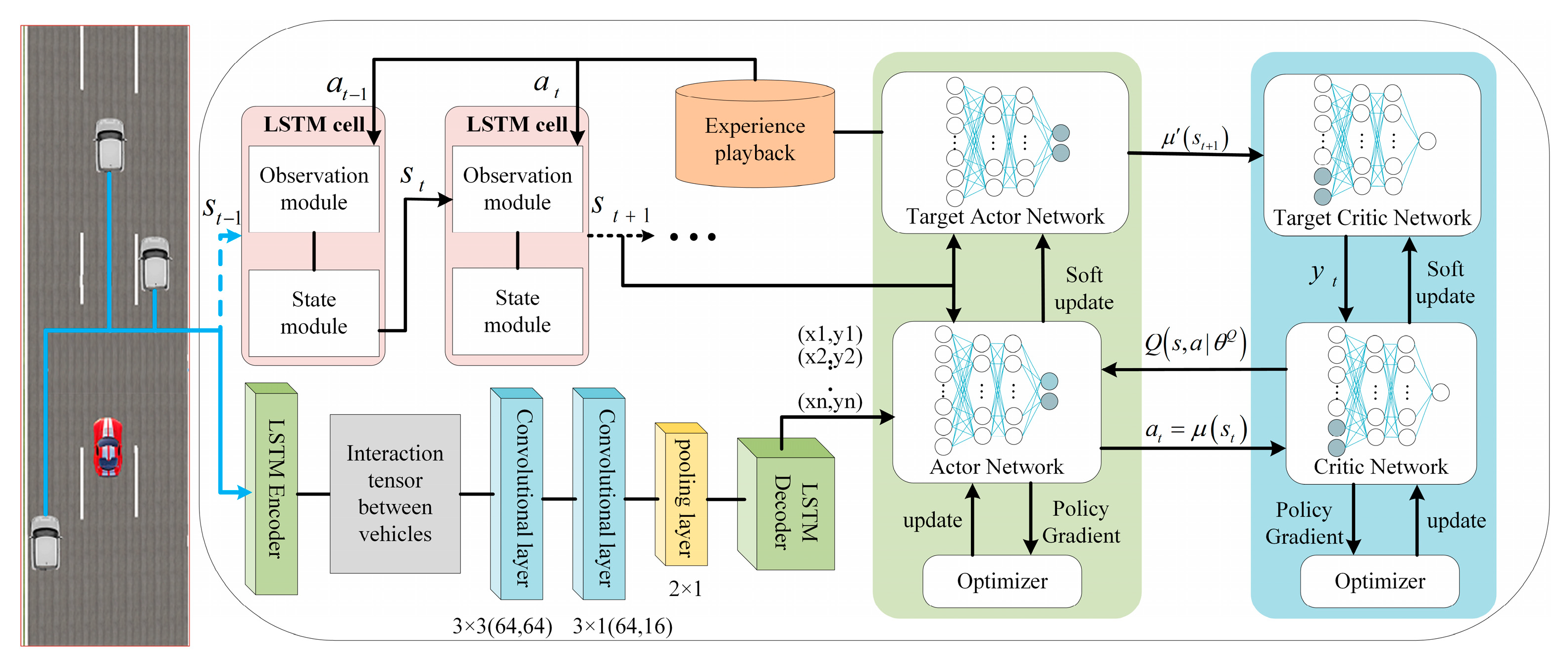
In this study, we integrated LSTM into the DDPG framework, resulting in LSTM-DDPG algorithm models, as illustrated in Figure 1. The LSTM is split into two branches. Each LSTM unit comprises an observation and a status module. The status module translates the observed values from the observation module into distinct status information. The second LSTM ingests the position data of the obstacle vehicle and, through the encoder, convolutional layer, and decoder, derives the anticipated trajectory information. The reinforcement learning component of LSTM-DDPG consists of both an actor network and a critic network, as depicted in Figure 1. Both the actor and critic networks employ a four-tiered structure, encompassing an input layer, an output layer, and two intermediate hidden layers. The hidden layers utilize the ReLU activation function to model the relationship between input and output signals.

The LSTM prediction model processes signals from various vehicle sensors, capturing the present state of the host vehicle and its surroundings. This model predicts the future trajectories of nearby vehicles. Using the forecasted trajectory combined with the current vehicle position, data are fed into the DDPG action network. The actor network then generates continuous action values for acceleration and the front wheel angle, based on an action strategy. Meanwhile, the critic network processes the state transformed by the LSTM along with the action output from the actor network, producing a return value. This return value is used to assess and continually refine the strategy of the actor network. Ultimately, the quintet of the current state, action, updated state, return value, and termination status is saved in the experience pool. Both actor and critic networks are refined using samples drawn from this pool.

The LSTM-DDPG algorithm pseudo-code is shown in

Table 1. LSTM-DDPG algorithm pseudo-code.

Algorithm: LSTM-DDPG
1	Initialize experience pool D
2	Initialize critic network ${\theta }^Q$, actor network ${\theta }^{\mu }$
3	Initialize target network ${\theta }^{Q^{-}}$, ${\theta }^{{\mu }^{-}}$
4	for episode in (1, M) do
5	set initial state S0
6	for t in (1, T) do
7	get the historical track X0 and Map to vector ${\mu }^t$
8	encode ${\mu }^t$ as an implicit state vector by encoder
9	predict the surrounding vehicle track Y0 by decoder
10	convert Y0 to location information and update st
11	select the optimal action at according to step 10 and action strategy
12	execute at and obtain current reward rt and observe next state $s_{t+1}$
13	store the element (si, ai, ri, st+1) in D
14	sample mini-batch (si, ai, ri, st+1) from D
15	update critic network using loss function L
16	update actor network using policy gradient ${\mathsf{\nabla }}_{{\theta }^{\mu }}\mu$
17	update the two target networks by soft update mode
18	end for
19	end for

.

3.2. Markov Process Modeling

3.2.1. Set State Space

During driving, the vehicle consistently interacts with its environment, maintaining a flow of state information. When making lane-changing decisions, it is crucial to consider the vehicle’s driving state and dynamics between the vehicle and its surroundings. In this study, the chosen state set incorporated information from both the host vehicle and road environment.

1.

The ego vehicle information on the road at time $t$, M[t] = {$v$, $d$, $x$, $\mathrm{y}$};

Ego vehicle information: The scalar input is chosen to represent the ego vehicle information using speed $v$ of the ego vehicle, distance $d$ between the ego vehicle and preceding vehicle, and ordinate ($x$, $\mathrm{y}$) of the ego vehicle trajectory.

2.

Predicted trajectories of surrounding vehicles on the road at time $t$;

LSTM was utilized to forecast the trajectories of neighboring vehicles. To uniformly represent the vehicle trajectory’s high-dimensional features, the historical trajectory coordinates of the surrounding vehicles at the given input time were transformed into word-embedding vectors using the fully connected layer ${\mu }^t$:

$${\mu }^t=FC\left(X^t; W_{\mathit{fc}}\right) ,$$

(1)

where FC() denotes a fully connected layer function, and $W_{\mathit{fc}}$ denotes the weight parameter of the fully connected layer.

The word-embedding vector of the corresponding vehicle historical trajectory and hidden state vector $h^{t-1}$ of the historical trajectory at the last moment were passed via the LSTM encoder to obtain the current hidden state vector $h^t$ containing the contextual information of the vehicle motion features:

$$h^t =\mathit{encoder}({\mu }^t,h^{t-1};W_{\mathit{enc}}),$$

(2)

where encoder() is responsible for encoding the word-embedding vector ${\mu }^t$ of the vehicle trajectory into an implicit state vector, and $W_{\mathit{enc}}$ denotes the weight parameter of the encoder.

Finally, the trajectory encoding the hidden state vector of all the vehicles around the current time is obtained as follows:

$$h_0^t,h_s^t\left(s\in \mathrm{1,2},\dots ,n\right) ,$$

(3)

Predicted trajectory: At any time $t$, the inputs of the trajectory prediction model are the trajectory coordinates of all vehicles $v_0$ around the host vehicle in the historical observation domain length $\mathit{his}$:

$$\begin{gathered} X_0=\left[\left(x_0^{t-\mathit{his}}, {\mathrm{y}}_0^{t-\mathit{his}}\right)\dots \left(x_0^{t-1}, {\mathrm{y}}_0^{t-1}\right),\left(x_0^t, {\mathrm{y}}_0^t\right)\right] \\ {X}_s=\left[\left(x_s^{t-\mathit{his}}, {\mathrm{y}}_s^{t-\mathit{his}}\right)\dots \left(x_s^{t-1}, {\mathrm{y}}_s^{t-1}\right),\left(x_s^t, {\mathrm{y}}_s^t\right)\right] , \end{gathered}$$

(4)

The model output comprises the coordinates of the driving trajectory of the target vehicle in the future prediction domain length pred:

$$Y_0=\left[\left(x_0^{t+1},{\mathrm{y}}_0^{t+1}\right)\dots \left(x_0^{t+2},{\mathrm{y}}_0^{t+2}\right),\left(x_0^{t+\mathit{pred}},{\mathrm{y}}_0^{t+\mathit{pred}}\right)\right] ,$$

(5)

3.2.2. Set Action Space

In the decision-making lane-changing problem of intelligent vehicles in this study, longitudinal velocity and lateral lane change need to be considered simultaneously. Therefore, we define the acceleration and steering wheel angle with continuous values as actor–network output A[t]: {a[t], δ[t]} [20].

Considering the longitudinal comfort of passengers, an acceleration output range within [–5, 5], and the tanh activation function were used in the output layer of the actor network to make the acceleration map output within [–1, 1]. Considering the actual situation of vehicle steering and lateral comfort of passengers, the wheel angle was limited in the range of [–30°, 30°], and finally, a tanh activation function was used to keep it within [–1, 1], which was convenient for model convergence. OU random processes with θ = 0.25 and σ = 0.2 are added to the output action to avoid a decrease in generalization ability due to sensing errors.

3.2.3. Design Reward Function

The actor network of the agent extracts the current status information from the LSTM module. It then selects an action from the action space according to its strategy and receives the corresponding reward (or penalty) based on this action. This interactive process continues until a termination condition is met. The agent’s goal is to achieve the maximum cumulative reward. Typically, the agent’s actions are assessed using a reward function. Hence, designing an apt reward function is crucial to the efficacy of the LSTM-DDPG algorithm. In this study, we designed a modular reward function that prioritizes safety, efficiency, and comfort.

1.

Safety

In terms of safety, autonomous vehicles must prioritize avoiding collisions with other vehicles on the road. It’s essential to guide the vehicle in selecting the appropriate driving lane. Specifically, if the vehicle chooses a positive steering wheel angle while in the left lane (indicating a lane change to the left) or a negative steering wheel angle in the right lane (indicating a lane change to the right), then these scenarios indicate an aberrant steering wheel angle. Consequently, a penalty value of −50 should be imposed in such instances. If a collision occurs during a lane change or while following another vehicle, a penalty of −200 should be assigned, ending the training. If the distance between vehicles falls below the safe margin given the current speed, then a penalty of −50 is imposed. In all other scenarios, a reward of +5 is given.

$$D_{\mathit{safe}}=vt+D_{-\mathit{default}} ,$$

(6)

where D_safe denotes the safe distance for the vehicle at a given speed, v denotes the current vehicle speed, t denotes the velocity coefficient, and D_-default denotes the initial safe distance.

$$r_1=\left\{\begin{array}{c}-200 if d<L_{vehicle} \\ -50 if d<D_{safe} \\ -50 if y>L_{lane}, \delta \ge 0, \\ -50 if y<L_{lane}, \delta \le 0 \\ +5 else \end{array} \right.$$

(7)

where d denotes the distance between the ego and preceding vehicles, $y$ denotes the lateral coordinate of the ego vehicle, $\delta$ denotes the front steering wheel angle of the ego vehicle, L_vehicle denotes the length of the ego vehicle, and L_lane denotes the length of the ego vehicle.

2.

Efficiency of Traffic

To ensure safety during lane changes, autonomous vehicles need to drive at an efficient pace without exceeding speed limits or changing lanes too frequently. Prolonged lane-changing maneuvers can reduce the efficiency of road usage, which would warrant a greater penalty.

$$r_2=-\mathrm{dt} ,$$

(8)

where dt denotes the simulation step size.

3.

Comfort

In the real driving process, frequent speed changes affect the comfort of passengers in a vehicle. Therefore, a reward function for lane-change comfort was designed according to vehicle acceleration and jerk.

$$r_3=\frac{1}{1+\left|a\right|+\left|\Delta a\right|} ,$$

(9)

where a denotes the acceleration of the vehicle, and $\Delta a$ denotes its jerk.

4.

Reward Function Ensemble

During the lane-change process, safety, lane-change efficiency, and comfort must be balanced. The total reward agent obtained for each time step is as follows:

$$R={\omega }_1{r}_1+{\omega }_2{r}_2+{\omega }_3{r}_3 ,$$

(10)

where ${\omega }_1$, ${\omega }_2$, ${\omega }_3$ denote the respective weight of the reward function involved in safety, lane-changing efficiency, and comfort. The safety weight mainly considers whether the vehicle complies with the traffic rules and whether there is a collision in the decision-making process. The weight of lane-change efficiency mainly considers the reasonable acceleration and deceleration in the process of vehicle running. The comfort weight mainly considers the acceleration and jerk of the vehicle. The greater the weight, the more the trained model emphasizes that particular factor. However, an excessively high weight can prevent the model from converging. The impact of the reward function on the policy network is intricate, and finding the optimal weight coefficient requires careful parameter tuning. Finally, weights for the reward function were designated as 5.0, 2.0, and 1.0.

3.3. Network Parameter Updating

DDPG consists of four networks: the online policy network, target policy network, online Q network, and target Q network, and the parameters of each network are updated alternately.

The critic network fits the action state value function according to the current state information $s_t$ and expected action ${\mu }_t$ generated by the actor network. To enhance the accuracy of the action value evaluation by the critic network, the online Q-network parameter value ${\theta }^Q$ is updated by minimizing the loss function, which can be defined as:

$$L=\frac{1}{n}\sum _i^n{(Q\left(s_i,{ a}_i|{\theta }^Q\right)-{\mathrm{y}}_i)}^2 ,$$

(11)

$${\mathrm{y}}_i=R_i+\gamma Q^{-}\left(s_i^{’},{\mu }^{-}\left(s_i^{’}|{\theta }^{{\mu }^{-}}\right)|{\theta }^{Q^{-}}\right) ,$$

(12)

where n denotes the sample number of the batch sampling experience, $R_i$ denotes the reward value of the experience sample $i$; $\gamma$ denotes the discount factor, ${\theta }^Q$ denotes the parameter of the online Q-network, ${\theta }^{Q^{-}}$ denotes the parameter of the target Q-network, Q$\left(s_i,{ a}_i|{\theta }^Q\right)$ denotes the action value estimated using the online critic network, and $Q^{-}\left(s_i^{’},{\mu }^{-}\left(s_i^{’}|{\theta }^{{\mu }^{-}}\right)|{\theta }^{Q^{-}}\right)$ denotes the future action value estimated using the target actor network and target critic network.

The actor network fits the policy function to generate the desired action ${\mu }_t$ based on the current state information $s_t$ of the model input, and the online policy network parameter ${\theta }^{\mu }$ updates the policy gradient expression as follows:

$${ \mathsf{\nabla }}_{{\theta }^{\mu }}\mu \approx \frac{1}{n}\sum _i{ \mathsf{\nabla }}_{{\theta }^{\mu }}\mu \left(s|{\theta }^{\mu }\right){|}_{s_i}{\mathsf{\nabla }}_{a}Q\left(s,a|{\theta }^Q\right){|}_{s_i,\mu \left(s_i\right)} ,$$

(13)

where $\mu \left(s|{\theta }^{\mu }\right)$ denotes a deterministic policy, and ${ \theta }^{\mu }$ denotes the online policy network parameter.

After each training iteration, gradients are utilized to update both online network parameters, while the target network parameters are updated using a soft update method. This method efficiently mitigates abrupt shifts and divergence in network gradient calculations, reduces large variations in network parameter updates, and promotes swift convergence during model training.

$$\begin{gathered} {\theta }^{{\mu }^{-}}=\tau {\theta }^{\mu }+\left(1-\tau \right){\theta }^{{\mu }^{-}} \\ {\theta }^{Q^{-}}=\tau {\theta }^Q+(1-\tau ){\theta }^{Q^{-}}, \end{gathered}$$

(14)

where ${ \theta }^{\mu }$, ${\theta }^{{\mu }^{-}}$ denote actor and target actor network parameters, respectively, ${\theta }^Q$, ${\theta }^{Q^{-}}$ denote critic and target critic network parameters, respectively, and τ denotes the soft update coefficient.

4. Verification of LSTM-DDPG Algorithm

In this study, we utilized the MATLAB R2021a simulation platform to establish simulation scenarios and algorithmic models. A representative two-lane highway setting was chosen to compare the LSTM-DDPG algorithm, which incorporates trajectory prediction, against the conventional Conv-DDPG algorithm that lacks this feature.

4.1. Training Scene Construction

When training the LSTM-DDPG algorithm, we should pay attention to the computational complexity of the algorithm. LSTM is a special recurrent neural network (RNN) whose computational complexity depends mainly on the depth and width of the network. Although the computational complexity of the LSTM in time steps is constant (O(1)), the overall computational burden increases as the number of network layers increases. The computational complexity of the DDPG mainly comes from updating the value function and optimizing the strategy. Therefore, the computational complexity of LSTM-DDPG will be the sum of the two, which can lead to challenges in real-time simulations. Considering the computational complexity of the LSTM-DDPG algorithm, the scenario shown in Figure 2 is set up.

Two training scenarios are selected to train the LSTM-DDPG algorithm. In scenario 1, there are two obstacle cars, whose positions are left behind and right in front. Scenario 2 has three obstacle vehicles, whose positions are left rear, left front, and right front. In the chosen scenario, the ego vehicle starts in the right lane. The position of the three obstacle cars is left rear, left front, and right ahead. However, the initial conditions of the obstacle vehicles (such as relative distance and speed in relation to the ego vehicle) adhere to specific constraints. The ego vehicle initiates at a speed of 65 km/h, with a maximum allowable speed of 100 km/h. The speed of obstacle car 1 is randomly generated in the range of 60–70 km/h, the speed of obstacle car 2 is randomly generated in the range of 70–80 km/h, and the speed of obstacle car 3 is randomly generated in the range of 60–70 km/h, and the initial distance from the car is 25 m.

During training, the initial parameters for the network training were set as follows: a learning rate of 0.005, batch size of 128, maximum of 500 iterations, and gradient threshold of 1. The Adam optimizer was chosen for the training process. The actor and critic networks in DDPG utilize a multi-layered fully connected structure. The actor network had neuron counts of 8, 256, 256, and 2, while the critic network comprised 10, 256, 256, and 1. The learning rates for the actor and critic networks were established at 0.001, and a discount factor of 0.99 was applied. Minibatch gradient descent was employed for training, with a batch size of 128 and cap of 1400 training epochs. The simulation operated at timesteps of 0.1 s.

4.2. LSTM Trajectory Prediction

4.2.1. Trajectory Preprocessing

In this study, we utilized MATLAB to design traffic scenarios on a straight roadway with varying densities: three cars and four cars. For each condition, the sequence of vehicle trajectory coordinates was captured at every time step to facilitate model training. The original data was captured at a frequency of 10 Hz, but was subsequently resampled at 5 Hz to ensure the retention of critical features in the dataset. For the processed data, an 8 s sliding window was employed to segment and generate data samples. Within this 8 s span, the initial 3 s served as historical data input to the model, while the succeeding 5 s acted as the reference for future trajectory predictions. The dataset was then categorized into training, validation, and testing subsets. Specifically, the initial 70% of samples were earmarked for training, the following 10% (from 70% to 80%) for validation, and the final 20% (from 80% to 100%) for testing.

Before employing the LSTM for trajectory prediction, it is essential to normalize the trajectory coordinates. This involves calculating the mean and standard deviation of the dataset and transforming it into a standardized dataset with a mean of one and variance of one. To better support the subsequent phased training of the LSTM network, datasets are stored using the cell-type data format.

To assess the accuracy of the predictions, the root−mean−square error (RMSE) was utilized to measure the deviation between the predicted and actual trajectories.

$$\mathit{RMSE}=\sqrt{\frac{1}{\mathit{pred}}\sum _{t=t_n+1}^{t_n+\mathit{pred}}{\delta }_t^T{\delta }_t},$$

(15)

$$\delta ={(x-{\mu }_x,\mathrm{y}-{\mu }_{\mathrm{y}})}^T,$$

(16)

where $t_n$ denotes the prediction start time, ($x$, $\mathrm{y}$) denote the coordinates of the real trajectory points, and the actual predicted trajectory coordinates are represented by the mean of the future trajectory distribution output (${\mu }_x$, ${\mu }_{\mathrm{y}}$) of the model.

4.2.2. Effect of Historical Duration

The appropriate input length for the LSTM network is crucial. If the input length is too brief, then it may not adequately capture the inherent mathematical characteristics of the data, leading to a significant decline in trajectory prediction accuracy. To delve deeper into how the duration of historical input trajectory impacts the extraction of vehicle interaction features by the trajectory prediction model, both qualitative and quantitative analyses of the model’s performance under varying input durations were conducted. The LSTM model was fed historical trajectory inputs of 1 s, 2 s, 3 s, 4 s, and 5 s. The RMSE values recorded during the training process are illustrated in Figure 3a. Upon analysis, the average RMSE values for the durations from 1 s to 5 s were 0.05457, 0.05324, 0.05115, 0.05067, and 0.05575, respectively.

Figure 3a demonstrates that the model begins to show signs of convergence around 50 steps for various input history lengths. As the input history field length ranged from 1 s to 4 s, there was a noticeable reduction in the deviation between the predicted and actual trajectories as the input historical trajectory of the model increased. This suggests that extending the historical trajectory can enhance the extraction of vehicle interaction features. However, when the length of the history field extended to 5 s, the predictive trajectory’s error began to increase, even surpassing the prediction inaccuracies observed at history field lengths of 1 s and 2 s. This indicates that an excessively long historical trajectory input may distort the interaction features the model seeks to extract. Analyzing the average RMSE value, the smallest error occurred at a model length of 4 s, indicating high predictive accuracy at this input length. Nevertheless, the prediction error for a 4 s input length was only marginally better than that for a 3 s input length, but it demanded more time and computational resources. When balanced against these factors, a history length of 3 s proved to be the most suitable model input.

As depicted in Figure 3b, the predicted vehicle trajectory coordinates align closely with the actual trajectory. The minimal prediction error suggests that the LSTM module developed in this study is effective in forecasting the genuine trajectory. Moreover, the trained encoder is well-suited for integration into the subsequent DDPG reinforcement learning decision-making model.

4.3. Comparison and Analysis

Based on the LSTM trajectory prediction module of the previous step, the representative states in the predicted trajectory and status module of the surrounding vehicles were considered as part of the input data of the LSTM-DDPG. During the simulation, the ongoing training episode was halted upon a collision with or overtaking of the lead vehicle. Subsequently, the virtual driving environment was reinitialized, and a fresh training episode commenced until the predefined training epochs were fulfilled.

Table 2. DDPG network structure.

Parameters	Layer	Dimension	Activation Function
Critic network	fully connected layer 1	(10, 256)	ReLU
	fully connected layer 2	(256, 256)	ReLU
	fully connected layer 3	(256, 1)	ReLU
Actor network	fully connected layer 1	(8, 256)	ReLU
	fully connected layer 1	(256, 256)	ReLU
	fully connected layer 1	(256, 2)	ReLU

and

Table 3. Training hyperparameter settings for DDPG.

Parameter	Parameter Values	Parameter	Parameter Values
Network learning rate	0.001	Sample size	64
Discount factor	0.99	Experience pool size	10,000
Gradient threshold	0.001	Maximum training period	1400

provide detailed information on the DDPG’s network architecture and hyperparameter settings.

In the DDPG algorithm’s learning journey, both episode reward and average reward serve as indicators of training convergence and the overall efficacy of learning. Figure 4a illustrates the training progression of the enhanced LSTM-DDPG. During the initial stages of training, the agent struggled to make appropriate lane-changing decisions. However, a significant surge in the average reward was observed between the 600th and 1000th training periods. Furthermore, this average reward largely remained consistent in the latter phases, suggesting that over time, the vehicle became adept at opting for actions with more favorable reward values, thus making better lane-changing choices.

It is necessary to balance safety, traffic efficiency, and comfort in lane-change decisions of autonomous vehicles. The curve of the average reward value normalized by a single step in the training process is smoothed, and the change curve is shown in Figure 4b. It can be observed that the reward value of the LSTM-DDPG algorithm gradually converges to 0.89 after about 1200 rounds of training. After about 1260 training rounds, the reward value of the Conv-DDPG algorithm gradually converges to 0.83. After about 1300 training rounds, the reward value of the TD3 algorithm gradually converges to 0.82. By comparison, it is found that the LSTM-DDPG algorithm has the fastest convergence speed, and the reward return is also improved.

As can be seen from Figure 4, with the continuous increase in the number of training rounds, the total reward value and the single-step reward value during training gradually become stable, which also reflects some indicators in the reward and punishment function. The reward and punishment functions are designed according to safety, traffic efficiency, and comfort, respectively. When the distance between the car and the front car, lane-changing situation of the car, speed, and acceleration of the car change greatly, the final reward value will be affected. Therefore, the stabilization of the reward value can reflect that the speed, acceleration, and traffic efficiency of the vehicle are also stable.

The average speed, average jerk value, and maximum steering wheel angle of the three algorithms in the process of lane change are shown in

Table 4. Comparison of algorithms.

	Average Velocity Speed (km/h)	Average Jerk Value (m·s−3)	Maximum Steering Wheel Angle (°)
LSTM-DDPG (Scenario1)	76.3	0.6	18.1
LSTM-DDPG (Scenario2)	77.5	0.7	18.1
Conv-DDPG	72.4	1.1	21.2
TD3	72.6	1.0	20.6

. It can be seen from the table that the LSTM-DDPG strategy algorithm performs better than the Conv-DDPG and TD3 strategy algorithm. The LSTM-DDPG strategy algorithm can change lanes with a smaller steering wheel angle, smaller jerk value, and higher speed, which not only ensures lane-change efficiency but also ensures comfort. The LSTM-DDPG strategy algorithm can run stably in different scenarios.

5. Conclusions

A lane-changing model was conceptualized using a Markov decision process. This model integrated LSTM-based trajectory predictions and pertinent state information into the actor–critic framework of the DDPG. Additionally, a multifaceted reward function specifically tailored for autonomous lane-changing was devised. Through iterative training guided by this reward function, the system can discern the optimal decision for autonomous lane-changing, considering the future state of vehicles it interacts with.

• Prediction of surrounding vehicles using LSTM: After the training of the data set, the LSTM module built can finally predict the relatively accurate future vehicle trajectory, and the prediction results are shown in Figure 3. At the same time as the state input of the DDPG algorithm, the vehicle can make better decisions on the lane-change trajectory.
• The LSTM-DDPG algorithm also performs well during training. As shown in Figure 4, both round reward and average reward increase significantly after the training cycle reaches 600 cycles. After the training cycle reaches 1000 cycles, the reward reaches an undetermined trend, and the vehicle can choose a better action to change lanes. The convergence speed of the LSTM-DDPG algorithm is faster than that of the Conv-DDPG algorithm.
• As can be seen from the data in Table 3, the LSTM-DDPG algorithm proposed in this paper can perform lane changes with faster speed and smaller acceleration in different scenarios. The vehicle can be more efficient and more comfortable while completing the task of a lane change.
• In the LSTM-DDPG algorithm, LSTM can help the DDPG algorithm capture and exploit this long-term dependency. When the driving scene changes, the LSTM-DDPG algorithm can update the strategy by learning the dynamic characteristics of the environment to provide continuous action space. The LSTM-DDPG algorithm may provide more robust decision strategies by learning long-term dependencies and continuous action spaces.