Do Sonic Tomography and Static Load Tests Yield Comparable Values of Load-Bearing Capacity?

Abstract

We tested the hypothesis that the loss of load-bearing capacity, as estimated by means of static load tests and from sonic tomography, is comparable. This is of practical importance for arborists when they have to assess results reported by different consultants or when they have to choose between applying one of these two methods in a specific case. A total of 59 trees, primarily Fagus sylvatica and Quercus robur, were subjected to static load tests and sonic tomography. The pulling test method yielded the residual stiffness of the stem at every position tested with a strain sensor as an intermediate quality parameter used to merely validate the actual estimations of safety against fracture. Based on the shape of the parts of the stem cross-section that are considered load bearing, sonic tomograms can be further processed in order to assess the loss of load-bearing capacity from defects like decay. We analyzed the correlation of these biomechanically equivalent parameters. This was only the case to a very limited extent. Sonic tomography and static load tests cannot replace each other, but they can complement each other.

1. Introduction

Property owners and government agencies have a legal duty of care for their trees and thus have to manage risks related to these trees. A central part of tree risk management is tree risk assessment. The main objective of assessing trees is to identify management strategies that ensure their longevity and optimal health, thus maximizing the benefits they provide. The risk posed by the vast majority of trees can be assessed visually during a basic assessment, but when a visual tree risk assessment reveals evidence of decay or other damage that might reduce the load-bearing capacity of a tree’s stem, arborists may use sonic tomography [1] or static load tests [2] for advanced tree inspections. These methods not only use different physical principles but also differ greatly in terms of effort and cost. For two reasons, arborists may need to know whether the use of both methods will lead to the same findings:

• If both methods are interchangeable, they could can the most cost efficient or practical method.
• When the same tree has been assessed using different methods by different consultants, they need to compare and evaluate the validity of the results.

This question has been studied before but with only limited sample sizes (six and seven trees, respectively) [3,4]. These studies came to contradictory results. While one found a very tight correlation, the other could not demonstrate any correlation between the results of the two methods.

Sometimes, far-reaching conclusions have been drawn from this hypothetical relationship, e.g., that these methods are interchangeable as they produce the same results. Especially due to the fact that the findings of advanced tree assessments are used to maintain safety in public spaces, a renewed investigation with a larger sample size seems warranted.

In this study, 59 trees were used to investigate whether sonic tomography and static load tests produce biomechanically comparable estimates of strength loss. For this purpose, the reduction in the section modulus due to internal defects was used, since this parameter can be estimated using both methods and thus compared objectively. While static load tests estimate the residual stiffness of the stem from the strain of the representative marginal fibers in bending, a loss of load-bearing capacity can be estimated from tomograms through photogrammetric analysis.

We tested the hypothesis that the residual stiffness estimated during the analysis of a static load test would correlate with the loss of load-bearing capacity estimated from tomograms.

2. Materials and Methods

In 2016, 23 pedunculate oaks (Quercus robur L.), 2 horse chestnuts (Aesculus hippocastanum L.), and 2 beech trees (Fagus sylvatica L.) with stem circumferences at 1 m height ranging from 208 cm to 671 cm were measured in a park in Hannover, Germany. In addition, 18 beech trees with stem circumferences between 250 cm and 450 cm were selected for inspection near Göttingen in 2019, as well as 8 sycamore maples (Acer pseudoplatanus L.), 2 red oaks (Quercus rubra L.), 2 lime trees (Tilia platyphyllos Scop.), and 2 wingnuts (Pterocarya fraxinifolia (Poir.) Spach) at different sites throughout Germany. Of these 59 trees, most were assessed because of evidence of decay.

The number and position of tomograms and strain measurements, as well as the number and directions of static load tests, depended on the individual damage and signs of decay of every tree. The tomograms were measured at one or two height levels per tree using a sonic tomograph and an electrical resistivity tomograph.

2.1. Tomography

Stress wave tomograms were taken with a Picus³ sonic tomograph (IML Electronic GmbH, Rostock, Germany), and electrical resistivity tomograms were taken with a Picus Treetronic³ (IML Electronic GmbH, Rostock, Germany).

Briefly, sonic tomographs measure the time-of-flight of signals excited by hammer blows and are recorded with 8–24 sensors attached with magnets to nails in one plane around the stem. The nails have to be in contact with the outermost growth ring. By tapping with a hammer on the nail at each measurement position, a network of apparent sonic velocities can be derived. The apparent stress wave velocity (v) is calculated from the time and distance data measured at the tree, assuming a straight path of the stress waves, because their true path is unknown. The resulting tomograms show apparent relative velocities and indicate the distribution of intact wood.

Electrical resistivity tomography can use the same nails as electrodes to inject and measure a current. Data were collected using a dipole–dipole configuration. The resulting tomograms show the distribution of apparent resistivity, which correlates with moisture and ion content [5,6,7] and thus allows for the location of cracks, decay, and cavities. Electrical resistivity tomography was used to provide additional information for easier interpretation of stress wave tomograms.

Sensor positions were recorded using an electronic caliper (Picus Caliper, IML Electronic, Rostock, Germany) with a system of triangulation.

Tomograms were produced with the software Picus Q74 (IML Electronic GmbH, Rostock, Germany). ERT inversion was based on [8,9], while the SoT-algorithm had not been documented by the manufacturer.

2.2. Static Load Tests

Static load tests were performed in one or two load directions. The instruments used were part of the TreeQinetic system (IML Electronic GmbH, Rostock, Germany). Up to four elastometers (strain meters) were mounted in the same planes that had been chosen for the sonic tomograms. During a static load test, force is exerted on the tree with a winch and a rope attached to the tree stem. While the winching tests were underway, the applied force was measured continuously with a force meter (load cell) in the pulling line, and the resulting strain (ε) in the stem was measured using several elastometers on the stem. Each elastometer spans 20 cm of the stem. The rope angle from the horizontal plane was measured using either a digital level on the tensioned rope or data provided by a built-in clinometer in the force meter. The applied force was converted into its lateral component by the cosine of the rope angle. The bending moment was determined as the product of the lateral force component (in kN) and the lever arm length as the vertical distance from the elastometers to the anchor point of the rope (in m).

From every test, only this part was used for evaluation when the force was slowly and steadily increased. Data were also stored during the release of the force but were not used for evaluation. In this way, it was possible to demonstrate that the trees were not damaged during the testing process. For every elastometer position, at least 100 pairs of force and elongation data were recorded and used for further data processing.

The static load tests were evaluated using Arbostat (Arbosafe GmbH, Gauting, Germany), and the residual stiffness of the cross-section E_R was derived. This parameter describes the flexural rigidity of the trunk actually measured in the static load tests using the strain ε recorded by the elastometers, compared to an intact trunk of this tree species with the stiffness E from the Stuttgart Strength Tables [2] and the section modulus W of an elliptical trunk cross-section with the stem diameter at the position of the elastometer:

$$E_R=\frac{M_B}{ϵEW}$$

(1)

where M_B is the applied bending moment during the pulling test.

In a standard application of the static load test method (SIM) [10], tree strength in bending would be assessed based on the extrapolation of measured strains during the pulling test to a critical strain, also termed the elastic limit or proportional limit of the fibers. Guideline values for this material property are available from the Stuttgart Strength Tables as well or can be derived from other specific tables on the mechanical properties of green wood [11,12,13,14]. During the evaluation process, the residual stiffness E_R merely serves as a control parameter which aims to compare the measured bending stiffness to the modulus of elasticity listed in tables.

The expected reduction in section modulus based on the sonic tomograms (Figure 1) was estimated using BoneJ [15] in ImageJ 1.54 software [16]. No material values had to be used for these purely geometric derivations from beam theory [17]. Only the brown areas of the tomograms were considered intact. While tomograms allow for the use of section moduli based on the real contour of the tree, for pulling tests, this is based on two perpendicular diameters and elliptic approximation.

Data were analyzed with the statistical program R [18], using robust linear models.

3. Results

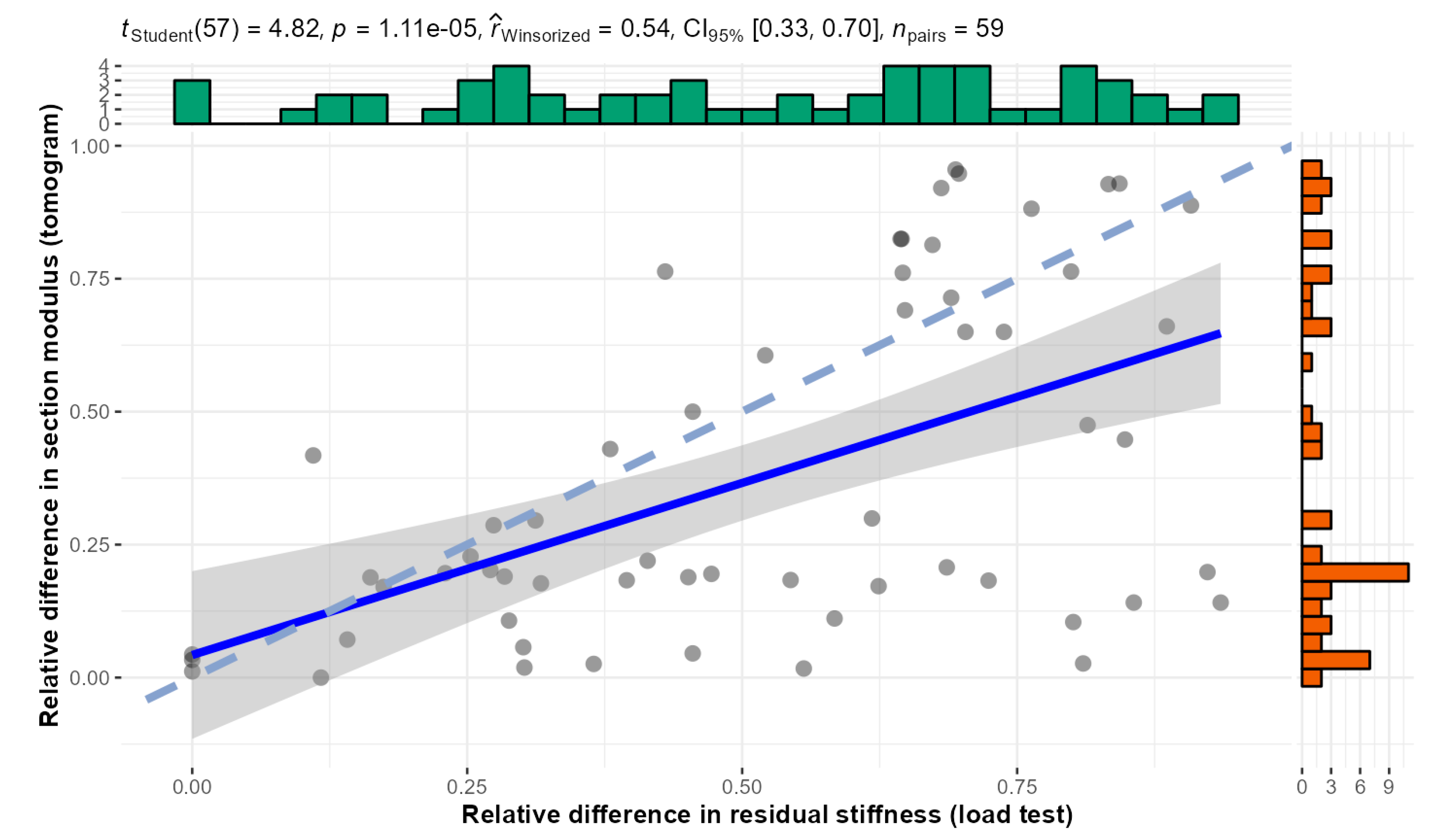
Pooling all species, a highly significant but loose correlation between the two strength loss parameters emerged (Figure 2), which almost exclusively occurred due to the data of beech (Figure 3), however. The residual stiffness estimated using the two methods was statistically highly significantly correlated for beech (correlation coefficient 0.56), and no relationship was detectable for oak (correlation coefficient ~0).

The section modulus W of the intact cross-section on which the evaluations of residual stiffness and loss of section modulus were based in the two methods differed considerably in some cases (Figure 4).

4. Discussion

Both sonic tomography and static load tests can produce estimates of the reduction in the section modulus of a tree stem. It seems reasonable to presume that the residual stiffness estimated during the analysis of a static load test would correlate with the loss of load-bearing capacity estimated from tomograms when placing instruments involving the use of both methods in the same plane of the trunk. Yet, overall, the correlation in our sample of trees was rather weak. For the species oak, it was not present at all.

Obvious causes are the assignment of the colors in the sonic tomograms to the categories “load bearing” and “no longer load-bearing”, as well as the highly simplified assumption of an elliptical trunk cross-section from which the residual stiffness is derived during the evaluation of the static load test.

When the flexural stiffness of a large stem with a complex shape, e.g., due to buttress roots, is approximated by the bending behavior of a cylinder with an elliptical cross-section, area may be added or subtracted at the periphery where fibers would strongly affect the stiffness of the beam. In addition, the two diameters used to calculate the ellipse, one in the direction of the load and the other perpendicular, will have a considerable range of variation: on large trees, the two axes can easily deviate from the right angle and from the horizontal plane. Moreover, there are sources of uncertainty that apply to all other diameter measurements. In fact, the beech trees were significantly smaller (mean diameter in the direction of load: 0.97 m ± 0.16 m) and more regularly shaped than the pedunculate oaks (mean diameter in the direction of load: 1.6 m ± 0.28 m), with there being significantly greater discrepancies between the two estimates. It may be suggested that the better fit for beech trees mainly occurred due to the more regular shape of their stems.

Any deviations in the actual elastic properties of wood from the values in the Stuttgart Strength Tables [2] would also affect the residual stiffness determined from Equation (1). Therefore, the residual stiffness E_R should not be used as an indicator for the extent of decay or strength loss directly. In our dataset, we did not find a reliable correlation between the residual stiffness calculated from the results of the pulling tests and the loss of section modulus in the tomograms. In the pulling test method, this parameter only serves as a control value to check the validity of the estimation of stem strength for obvious errors, e.g., due to false positioning of the elastometer on dead wood. For the present study, all deviations of the measured flexural stiffness are attributed to changes in the section modulus, whereas the effects of a simplified elliptical shape and the actual wood properties were neglected in order to replicate the methods used in [3,4].

The distribution of load-bearing wood fibers within the cross-section strongly affects the strength and flexibility in bending. Furthermore, the degree of decay may change the elastic properties of wood at different positions of the cross-section [3], based on [19], with weighted areas of tomograms based on sound velocities. This approach has significant limitations. It is based on the assumption that a tight and linear correlation exists between sound velocities depicted for a specific location in a tomogram and the actual properties of the wood fibers at that location. However, this correlation is typically quite low [20,21] because tomograms show estimates of apparent stress wave velocities between sensor positions on the periphery of the stem, presuming linear stress wave propagation. Actually, stress waves are more likely to travel around decayed sections rather than pass through them. Therefore, the tomogram also depicts the properties of the sections of the stem cross-section without direct measurements [1].

Furthermore, there is considerable variation and systematic trends in wood density, modulus of elasticity (MOE), modulus of rupture (MOR), and stress-wave velocity in stem cross-sections, not only between different species but also within and between trees [22,23,24,25,26,27,28,29]. In severely decayed trees, such as those in this study, this variability may be even greater, as damaged wood has been shown to be much tougher than normal wood [30]. Even under ideal conditions, the correlation between stress wave velocity and the modulus of rupture can be quite low [25,31,32,33]. Wood is an anisotropic material with a different material response depending on the direction of the applied stress. The tomographic inversion we used does not take into account that the stress wave velocity was measured in all directions between radial and tangential, adding another source of variation. Several studies have shown that velocity alone, assuming a constant wood density, is not sufficient for accurate estimates of wood’s physical properties [34,35]. Although desirable to increase the accuracy of the estimate, it is clear that weighing the contribution of tomographic pixels to the load-bearing capacity with the stress wave velocity, as described by [19], would not be justified. Another point of debate is the best color threshold to use to discriminate between intact wood and decay or cavities [36,37]. Based on our experience, we decided not to include green areas in the decay/cavity category.

The strength loss assessment we used assumes a homogeneous and isotropic material with the same MOE in compression and tension. This assumption is likely to be violated in wood [38]. Another parameter that affects the results of static load tests but is neglected in strength loss calculations solely based on the distribution of intact wood is pre-strains, which could increase the safety of the tree [39].

Another reason for the sometimes large differences between the results of the two methods may be cracks in the log cross-section, which can lead to large areas in the stress wave tomogram that are no longer considered load bearing, even though they are still largely intact. Cracks act like barriers for stress wave propagation and force them to deviate from a linear direction. As the time of flight thus increases, the area behind a crack may be illustrated in a tomogram just like a decayed section.

However, there is an important difference in how the estimated reduction in load-bearing capacity is used within the two different methods. In the static load test method, the residual stiffness is merely a control variable that has no effect on the result of the investigation and thus the ultimate risk assessment. It only serves to detect false sensor placement, sensor malfunction, or deviations in the material properties of the specimen tree from the guideline values [2]. Yet, an evaluation of stem strength is often based on the loss of bearing capacity derived from tomograms [36,40]. Given the fact that even small changes in the shape of a cross-section may result in large differences in section modulus, especially in the periphery of the cross-section, the results re-emphasize the need to record the positions of the sensors as accurately as possible during tomography, not only in order to avoid the misinterpretation of time of flight signals [41,42,43] but also to correctly assess the section modulus for an estimate of strength loss. Otherwise, significant misinterpretations of fracture safety must be anticipated in light of the current findings. On the contrary, in the static load test method, incorrect estimates of residual stiffness will not result in false interpretations of load-bearing capacity because fracture safety is estimated based on strain measurements alone [2].

Already, an earlier attempt to reproduce the results of [4] could not confirm them [3]. Also, in the present study, the very tight linear relationship found by [4] between the residual stiffness derived from static load tests and the loss of section modulus estimated from the photogrammetric analysis of sonic tomograms could not be confirmed.

5. Conclusions

Sonic tomography and static load tests cannot replace each other, but they can complement each other. For example, tomography can help to determine the best load direction before a static load test is undertaken. After the static load test, tomography can provide a significant contribution to the prediction of the further development of damage, e.g., resulting from decay.

A tomogram can also be used to better select reference values for wood properties in static load tests. Despite the fact that radial stress wave propagation cannot predict wood properties in the axial direction, it may be possible to demonstrate that the stem has no hidden damage. If the stem has a rather regular elliptical shape, the apparent modulus of elasticity measured with strain sensors during the static load test can be used to adapt elastic wood properties for the evaluation of the test.

On the other hand, static load tests can be used to verify the results of tomography with respect to the actual deformation of the representative fibers in the periphery of the stem. Due to the inclusion of a wind load estimate in the analysis of static load tests, the assessment of fracture safety is based not only on a measure of relative strength loss compared to an intact section but also on the safety reserves that a mature tree may have accumulated, for example, by increasing its stem diameter before any major damage occurs to the load-bearing structure and as it continuously compensates for such damages by adaptively increasing its annual incremental growth.

References

- Rust, S. A New Tomographic Device for the Non-Destructive Testing of Standing Trees. In Proceedings of the 12th International Symposium on Nondestructive Testing of Wood, University of Western Hungary, Sopron, Hungary, 13–15 September 2000; pp. 233–238. [Google Scholar]
- Wessolly, L.; Erb, M. Manual of Tree Statics and Tree Inspection; Patzer Verlag: Berlin, Germany, 2016; ISBN 978-3-87617-143-2. [Google Scholar]
- Wolf, J. Experimentelle Überprüfung der Berechnung der Flächenträgheitsmomente aus dem Impulstomogramm. Bachelor’s Thesis, Hochschule Bremen, Bremen, Germany, 2010. [Google Scholar]
- Lesnino, G. Vergleichsuntersuchungen zur Sicherheitsermittlung an Bäumen—Schalltomografie und Zugversuche. In Proceedings of the Baumtage Süd, Böblingen, Germany, 20–21 October 2009; pp. 1–5. [Google Scholar]
- Bieker, D.; Kehr, R.; Weber, G.; Rust, S. Non-Destructive Monitoring of Early Stages of White Rot by Trametes Versicolor in Fraxinus Excelsior. Ann. For. Sci. 2010, 67, 210. [Google Scholar] [CrossRef]
- Bieker, D.; Rust, S. Non-Destructive Estimation of Sapwood and Heartwood Width in Scots Pine (Pinus sylvestris L.). Silva Fenn. 2010, 44, 267–273. [Google Scholar] [CrossRef]
- Bieker, D.; Rust, S. Electric Resistivity Tomography Shows Radial Variation of Electrolytes in Quercus Robur. Can. J. For. Res. 2010, 40, 1189–1193. [Google Scholar] [CrossRef]
- Günther, T.; Rücker, C.; Spitzer, K. Three-Dimensional Modelling and Inversion of Dc Resistivity Data Incorporating Topography—II. Inversion. Geophys. J. Int. 2006, 166, 506–517. [Google Scholar] [CrossRef]
- Just, A.; Jacobs, F. Elektrische Widerstandstomographie zur Untersuchung des Gesundheitszustandes von Bäumen. In Proceedings of the VII. Arbeitsseminar “Hochauflösende Geoelektrik”, Bucha, Germany, 3–5 November 1998; Danckwardt, E., Ed.; Institut für Geophysik und Geologie der Universität Leipzig: Bucha, Germany, 1998. [Google Scholar]
- Sinn, G.; Wessolly, L. A Contribution to the Proper Assessment of the Strength and Stability of Trees. Arboric. J. 1989, 13, 45–65. [Google Scholar] [CrossRef]
- Niklas, K.J.; Spatz, H.-C. Worldwide Correlations of Mechanical Properties and Green Wood Density. Am. J. Bot. 2010, 97, 1587–1594. [Google Scholar] [CrossRef] [PubMed]
- Kretschmann, D.E. Chapter 5 Mechanical Properties of Wood. In Wood Handbook General Technical Report FPL–GTR–190; Forest Products Laboratory: Madison, WI, USA, 2010. [Google Scholar]
- Jessome, A.P. Strength and Related Properties of Woods Grown in Canada; Eastern Forest Products Laboratory: Ottawa, ON, Canada, 1977. [Google Scholar]
- Lavers, G.M.; Moore, G.L. The Strength Properties of Timber; Department of the Environment, Building Research Establishment; HMSO: Watford, UK, 1983. [Google Scholar]
- Doube, M.; Kłosowski, M.M.; Arganda-Carreras, I.; Cordelières, F.P.; Dougherty, R.P.; Jackson, J.S.; Schmid, B.; Hutchinson, J.R.; Shefelbine, S.J. BoneJ: Free and Extensible Bone Image Analysis in ImageJ. Bone 2010, 47, 1076–1079. [Google Scholar] [CrossRef] [PubMed]
- Schindelin, J.; Arganda-Carreras, I.; Frise, E.; Kaynig, V.; Longair, M.; Pietzsch, T.; Preibisch, S.; Rueden, C.; Saalfeld, S.; Schmid, B.; et al. Fiji: An Open-Source Platform for Biological-Image Analysis. Nat. Methods 2012, 9, 676–682. [Google Scholar] [CrossRef]
- Koizumi, A.; Hirai, T. Evaluation of the Section Modulus for Tree-Stem Cross Sections of Irregular Shape. J. Wood Sci. 2006, 52, 213–219. [Google Scholar] [CrossRef]
- R Core Team. R: A Language and Environment for Statistical Computing; R Foundation for Statistical Computing: Vienna, Austria, 2021. [Google Scholar]
- Rinntech. Benutzerhandbuch Arbotom; Rinntech: Heidelberg, Germany, 2011. [Google Scholar]
- Cristini, V.; Tippner, J.; Tomšovský, M.; Zlámal, J.; Mařík, R. Acoustic Tomography Outputs in Comparison to the Properties of Degraded Wood in Beech Trees. Eur. J. Wood Prod. 2022, 80, 1377–1387. [Google Scholar] [CrossRef]
- Bork, R.; Düsterdiek, S.; Detter, A.; Rust, S. Vergleich von Zugversuchen, Materialtests an Kleinproben und Literaturwerten. In Proceedings of the Jahrbuch der Baumpflege; Dujesiefken, D., Ed.; Haymarket Media: Augsburg, Germany, 2012; pp. 237–242. [Google Scholar]
- Gil-Moreno, D.; MClean, J.P.; Ridley-Ellis, D. Models to Predict the Radial Variation of Stiffness, Strength, and Density in Planted Noble Fir, Norway Spruce, Western Hemlock, and Western Red Cedar in Great Britain. Ann. For. Sci. 2023, 80, 1–15. [Google Scholar] [CrossRef]
- Lachenbruch, B.; Moore, J.R.; Evans, R. Radial Variation in Wood Structure and Function in Woody Plants, and Hypotheses for Its Occurrence. In Size- and Age-Related Changes in Tree Structure and Function; Meinzer, F.C., Lachenbruch, B., Dawson, T.E., Eds.; Tree Physiology; Springer: Dordrecht, The Netherlands, 2011; Volume 4, pp. 121–164. ISBN 978-94-007-1241-6. [Google Scholar]
- Schimleck, L.R.; Dahlen, J.; Auty, D. Radial Patterns of Specific Gravity Variation in North American Conifers. Can. J. For. Res. 2022, 52, 889–900. [Google Scholar] [CrossRef]
- Van Duong, D.; Hasegawa, M.; Matsumura, J. The Relations of Fiber Length, Wood Density, and Compressive Strength to Ultrasonic Wave Velocity within Stem of Melia Azedarach. J. Indian Acad. Wood Sci. 2019, 16, 1–8. [Google Scholar] [CrossRef]
- Rungwattana, K.; Hietz, P. Radial Variation of Wood Functional Traits Reflect Size-Related Adaptations of Tree Mechanics and Hydraulics. Funct. Ecol. 2018, 32, 260–272. [Google Scholar] [CrossRef]
- Wassenberg, M.; Chiu, H.-S.; Guo, W.; Spiecker, H. Analysis of Wood Density Profiles of Tree Stems: Incorporating Vertical Variations to Optimize Wood Sampling Strategies for Density and Biomass Estimations. Trees 2015, 29, 551–561. [Google Scholar] [CrossRef]
- Ubuy, M.H.; Eid, T.; Bollandsås, O.M. Variation in Wood Basic Density within and between Tree Species and Site Conditions of Exclosures in Tigray, Northern Ethiopia. Trees 2018, 32, 967–983. [Google Scholar] [CrossRef]
- Bouslimi, B.; Koubaa, A.; Bergeron, Y. Regional, Site, and Tree Variations of Wood Density and Growth in Thuja occidentalis L. in the Quebec Forest. Forests 2022, 13, 1984. [Google Scholar] [CrossRef]
- Kane, B.C.P.; Ryan, H.D.P.I. Examining Formulas That Assess Strength Loss Due to Decay in Trees: Woundwood Toughness Improvement in Red Maple (Acer rubrum). J. Arboric. 2003, 29, 209–217. [Google Scholar] [CrossRef]
- Duong, D.V.; Schimleck, L.; Tran, D.L.; Vo, H.D. Radial and Among-Clonal Variations of the Stress-Wave Velocity, Wood Density, and Mechanical Properties in 5-Year-Old Acacia Auriculiformis Clones. BioResources 2022, 17, 2084–2096. [Google Scholar] [CrossRef]
- Lachenbruch, B.; Johnson, G.R.; Downes, G.M.; Evans, R. Relationships of Density, Microfibril Angle, and Sound Velocity with Stiffness and Strength in Mature Wood of Douglas-Fir. Can. J. For. Res. 2010, 40, 55–64. [Google Scholar] [CrossRef]
- Papandrea, S.F.; Cataldo, M.F.; Bernardi, B.; Zimbalatti, G.; Proto, A.R. The Predictive Accuracy of Modulus of Elasticity (MOE) in the Wood of Standing Trees and Logs. Forests 2022, 13, 1273. [Google Scholar] [CrossRef]
- Watt, M.S.; Trincado, G. Modelling between Tree and Longitudinal Variation in Green Density within Pinus Radiata: Implications for Estimation of MOE by Acoustic Methods. N. Z. J. For. Sci. 2014, 44, 16. [Google Scholar] [CrossRef]
- Todoroki, C.L.; Lowell, E.C. Validation of Models Predicting Modulus of Elasticity in Douglas-Fir Trees, Boles, and Logs. N. Z. J. For. Sci. 2016, 46, 11. [Google Scholar] [CrossRef]
- Burcham, D.C.; Brazee, N.J.; Marra, R.E.; Kane, B. Can Sonic Tomography Predict Loss in Load-Bearing Capacity for Trees with Internal Defects? A Comparison of Sonic Tomograms with Destructive Measurements. Trees-Struct. Funct. 2019, 33, 681–695. [Google Scholar] [CrossRef]
- Brazee, N.J.; Burcham, D.C. Internal Decay in Landscape Oaks (Quercus Spp.): Incidence, Severity, Explanatory Variables, and Estimates of Strength Loss. Forests 2023, 14, 978. [Google Scholar] [CrossRef]
- Langum, C.E.; Yadama, V.; Lowell, E.C. Physical and Mechanical Properties of Young-Growth Douglas-Fir and Western Hemlock from Western Washington. For. Prod. J. 2009, 59, 37–47. [Google Scholar] [CrossRef]
- Bonser, R.H.C.; Ennos, A.R. Measurement of Prestrain in Trees: Implications for the Determination of Safety Factors. Funct. Ecol. 1998, 12, 971–974. [Google Scholar] [CrossRef]
- Rinn, F. Statische Hinweise im Schall-Tomogramm von Bäumen. Stadt Und Grün 2004, 7, 41–45. [Google Scholar]
- Rust, S. Accuracy and Reproducibility of Acoustic Tomography Significantly Increase with Precision of Sensor Position. J. For. Landsc. Res. 2017, 2, 1–6. [Google Scholar] [CrossRef]
- Rust, S. Reproducibility of Stress Wave and Electrical Resistivity Tomography for Tree Assessment. Forests 2022, 13, 295. [Google Scholar] [CrossRef]
- Burcham, D.C.; Brazee, N.J.; Marra, R.E.; Kane, B. Geometry Matters for Sonic Tomography of Trees. Trees 2023, 37, 837–848. [Google Scholar] [CrossRef]
Figure 1.
Example of a tomogram of Tilia cordata. Brown indicates high apparent stress wave velocity and thus sound wood, while green, red, and blue indicate decreasing levels of velocity. Axes are scaled in cm.
Figure 2.
Correlation between the bearing capacity losses measured using different methods, with relative values based on a comparison to the intact cross-section. Slope 0.66 ± 0.1. Blue line: linear regression with confidence interval (gray). Dashed line 1:1.
Figure 3.
Correlation between the bearing capacity losses measured using different methods for two species with large sample sizes ((a): F. sylvatica; (b): Quercus robur), with relative values based on the comparison with the intact cross-section. Blue lines: linear regression with confidence interval (gray).
Figure 4.
Correlation between the section moduli W of the intact cross-sections used for tomograms and static load tests. Slope 0.77 ± 0.05. Blue line: linear regression with confidence interval (gray). Dashed line 1:1.
Disclaimer/Publisher’s Note: The statements, opinions and data contained in all publications are solely those of the individual author(s) and contributor(s) and not of MDPI and/or the editor(s). MDPI and/or the editor(s) disclaim responsibility for any injury to people or property resulting from any ideas, methods, instructions or products referred to in the content. |
© 2024 by the authors. Licensee MDPI, Basel, Switzerland. This article is an open access article distributed under the terms and conditions of the Creative Commons Attribution (CC BY) license (https://creativecommons.org/licenses/by/4.0/).
Share and Cite
MDPI and ACS Style
Rust, S.; Detter, A. Do Sonic Tomography and Static Load Tests Yield Comparable Values of Load-Bearing Capacity? Forests 2024, 15, 768. https://0-doi-org.brum.beds.ac.uk/10.3390/f15050768
AMA Style
Rust S, Detter A. Do Sonic Tomography and Static Load Tests Yield Comparable Values of Load-Bearing Capacity? Forests. 2024; 15(5):768. https://0-doi-org.brum.beds.ac.uk/10.3390/f15050768
Chicago/Turabian StyleRust, Steffen, and Andreas Detter. 2024. "Do Sonic Tomography and Static Load Tests Yield Comparable Values of Load-Bearing Capacity?" Forests 15, no. 5: 768. https://0-doi-org.brum.beds.ac.uk/10.3390/f15050768
Note that from the first issue of 2016, this journal uses article numbers instead of page numbers. See further details here.