

A Comparison of Different Biomass Combustion Mechanisms in the Transient State

1
ECT-UTAD School of Science and Technology, University of Trás-os-Montes e Alto Douro, 5000-801 Vila Real, Portugal
2
INEGI/LAETA Mechanical Engineering Department, Faculty of Engineering, University of Porto, 4099-002 Porto, Portugal
3
MEAM Department of Mechanical Engineering and Applied Mechanics, School of Engineering, University of Pennsylvania, Philadelphia, PA 19104, USA
*
Author to whom correspondence should be addressed.
Energies 2024, 17(9), 2092; https://0-doi-org.brum.beds.ac.uk/10.3390/en17092092
Submission received: 12 March 2024
/
Revised: 30 March 2024
/
Accepted: 23 April 2024
/
Published: 27 April 2024
(This article belongs to the Section A4: Bio-Energy)
Abstract
:Different combustion reaction process models were used to numerically study the behavior of the temperature, velocity, and turbulence fields, as well as to gain a better understanding of the differences between the reaction products obtained with each model. Transient-state simulations were conducted for a gasifier under specific operating conditions. The standard K-epsilon (2eq) turbulence model was utilized, along with the incorporation of species transport, volumetric responses, and eddy dissipation. In this study, the impacts of one-, two-, and four-step reaction mechanisms on the mass fraction of the products of the reactions, as well as the maximum values of velocity, turbulence, and temperature, were examined. The findings demonstrated that for all mechanisms, the greater maximum values of velocity and turbulence are attained at early time steps and decrease with subsequent time steps. The temperature rises as much in the early time steps and nearly stays the same in the late time steps. In all situations examined, the species’ fraction mass varies slightly in the early time steps but becomes nearly constant in the latter time stages. Similar species mass fraction values were found for both one-step and four-step methods. The results also suggest that the lower half of the gasifier is where the highest mass fraction values are found.
Keywords:
biomass; CFD; turbulent model; transient state; species transport; eddy dissipation; combustion1. Introduction
In the past few decades, the demand for energy sources has increased and continues to increase today. From 1971 to 2014, global energy usage increased by 44%, with 80% of the energy being produced using fossil fuel resources [1]. This massive increase in the usage of fossil fuel resources leads to environmental problems, with carbon emissions leading to an increase in global warming. To lower CO2 emissions and avoid environmental degradation, the utilization of renewable energy sources was proposed [2,3].
The growing recognition of the environmental problems associated with the usage of fossil fuels increased the demand for alternative energies in the 21st century [4]. In the past decade, the world’s primary energy consumption has been met by the use of renewable energy sources. In 2012, the primary energy consumption of renewable energy was 2%, but this value increased to 6.7% in 2021 [5].
Some studies have shown that the utilization of biomass to produce energy is an attractive approach because it presents lower environmental impacts than fossil fuels, and carbon dioxide can be considered neutral as this gas is consumed during growth. Biomass is an organic substance that appears in nature in different shapes and sizes [6].
Biomass fuels can be categorized into six primary classes: wood and woody materials (hard and soft wood, etc.), herbaceous fuels (straw, grasses, etc.), wastes (sewage sludge, refuse-derived fuel (RDF), etc.), derivates such as waste from industries, aquatic (kelp, etc.), and energy crops (cultivated for energy purposes) [7,8].
Biomass can be used to produce energy using different thermochemical conversion technologies like pyrolysis, combustion, gasification, and liquefaction [9]. However, using these types of technologies can be pricy because of the equipment required and storage.
On the other hand, CFD modeling has become increasingly important since it is a more economical tool that can be used to study the combustion of biomass because it can provide a better understanding of this conversion technique and possibly optimize it [10,11].
A mathematical description of combustion can be complex because fluid mechanics, mass transfer, chemical kinetics, and thermodynamics must all be accounted for. For CFD models, the fluid mechanic and thermodynamic conservation equations, such as mass, momentum, and energy, need to be satisfied or else the model cannot be considered valid [6].
Modeling CFD models with biomass can be a challenge due to the complexity of the biomass. The combustion of biomass is heavily influenced by the proprieties of the feedstock and chemical reactions [12].
Some reviews on the topic of biomass combustion indicate that there are several models that can be used, and it is up to the user to choose which one is the best for a certain application. Tabet and Gökalp [10] and Marangwanda et al. [6] presented an overview of CFD models for co-combustion under air and oxy-fuel conditions and combustion, respectively. The overviews mention that current CFD models can solve complex processes.
The model proposed by Jones and Lindstedt (JL) [13] is commonly used for combustion modeling for air–fuel applications. Yin et al. [14] refined the model proposed by JL for biomass co-firing under oxy-fuel conditions. The main difference is that the refined model uses the H2 oxidation model proposed by Marinov et al. [15].
Yin et al. [16] investigated the combustion characteristics of pure coal and wheat straw in a swirl-stabilized burner, and Álvarez et al. [17] studied the co-combustion of olive waste with different coals under three different oxy-fuel conditions. These studies revealed that the JL model is a good option for modeling biomass combustion because it can help accurately predict the major species produced and the gas temperature.
Medina et al. [18] performed a numerical study to calculate CO2 mass flow rates and thermal and combustion efficiency for a plancha-type cookstove by using a one-step reaction mechanism. The results obtained showed that CO2 mass flow rates had a good correlation with experimental results.
With continuous industrial development, in recent years, CFD studies have been primarily focused on bubble morphology [19], mixing mass transfer [20], and power measurements [21]. Ge and Zheng [22] proposed a fluid–solid mixing tank to improve the mixing efficiency and quality in chemical engineering and lithium battery production. Li et al. [23] proposed a real-time sensing method using MFSV-induced vibration that can be helpful for fluid-induced vibration detection and industrial monitoring systems.
The main objective of this study is to compare and quantify the numerical results of the combustion models to understand the implications of choosing each one of them in validating the comparison between different studies available in the literature. For this, an investigation of the influence of the choice of combustion model in a transient regime on the flow within a gasifier under specific conditions was carried out. The three combustion models analyzed use different reaction mechanisms (one step, two steps, and four steps). CFD simulations were performed to study the mass fraction in the composition of the gas created, as well as the behavior of velocity, temperature, and turbulence.
2. Materials and Methods
In this study, a 2D geometry of a gasifier was used to perform the simulations with the Ansys Fluent software. The Ansys Fluent software was chosen because it is a software that stands out as one of the most used in this type of study, e.g., [24,25,26]. In Figure 1, we can see that the gasifier has two side inlets and two outlets (one at the top and one at the bottom). The wood and air are introduced in the two side inlets, and the products of the combustion leave through the two outlets.
To perform the simulation, the K-epsilon (2eq) standard turbulence model was chosen because it is one of the simplest models and is used in similar studies present in the literature, e.g., [24]. The species transport and the volumetric reactions with eddy dissipation were activated, and the wood–volatile–air was chosen. The eddy dissipation acknowledges that the chemical kinetic rate (chemical reaction) is faster than the rate of turbulent mixing. Due to the turbulent nature of the combustion, the eddy properties give information concerning the mixing time [6].
The discrete phase model (DPM) was turned on since CFD codes utilize DPM to capture the multiphase processes of the solid and gaseous phases present in this study. This model (DPM) will consider how the gaseous components (continuum phase) will interact with the solid particles (discrete phase) present during the combustion process [6]. It was decided that the particles would only be injected at the start (time equal to 0 s) with a velocity of 0.6 m/s and a temperature of 300 K. For the particle type, the combusting condition was chosen, and for the injection type (inlet), the surface condition was chosen. The numerical solutions were obtained using the coupled method with a courant number of 1.
For the boundary conditions, a velocity condition was imposed for the inlets (velocity-inlet) with a velocity of 0.6 m/s and a temperature of 300 K. A turbulent intensity of 10% and a viscosity ratio of 10 were also imposed. For the outlets, a pressure condition (pressure-outlet) was used, which makes the pressure in the outlets equal to the atmospheric pressure. On the walls, a non-slip condition was used, and it was considered that the walls are adiabatic, so no heat or matter exchanges will occur between the system and the surrounding environment, with a temperature of 300 K. The simulation does not take into account radiative heat transfer between the system and its surroundings.
During the conversion processes, some species are released into a gaseous phase (volatiles, CO, CO2, etc.), creating sources for gas phase combustion [17]. The volatiles will, most times, carry a large percentage of the energy of solid fuels, for example, around 50% for coals and an even larger amount for biomass. So, the homogeneous combustion of the volatiles plays an important role in flame stability and ignition, local temperature, distribution of species, and pollutant formation. Therefore, gas–solid combustion mechanisms are expected to play an important role in modeling the combustion process.
In CFD, the volatiles are combined into a single “artificial” species, usually represented as CHyOz [6].
In this study, “1-step”, “2-step”, and “4-step” reactions were used. The labels “1-step”, “2-step”, and “4-step” represent a 1-step global reaction, which will have CO2 (carbon dioxide) and H2O (water) as products; 2-step global reactions with CO (carbon monoxide), CO2, and H2O as products; and 4-step global reactions with CO, H2 (hydrogen), CO2, and H2O as products, respectively.
The 1-step reaction is a simple equation without any intermediate species. The global one-step reaction mechanism used is
CH2.382O1.075 + 1.058 O2 → CO2 + 1.191 H2O
The 2-step reaction is considered a more accurate approach (compared to a 1-step reaction), having carbon monoxide as an intermediate species. The global two-step reaction mechanism used, derived from the mechanism proposed by Westbrook and Dryer [10,27], is
CH2.382O1.075 + 0.558 O2 → CO + 1.191 H2O
CO + 0.5 O2 → CO2
Another mechanism (4-step reaction) was proposed by JL and then refined by Yin et al. [14] to improve the accuracy of the volatile combustion. These 4 reactions are enough to perform a detailed study of the combustion process. In comparison with the original JL mechanism, the refined mechanism retains the initial reactions involving hydrocarbon and O2 but refines the CO-CO2 reactions [10,17]. The global four-step reaction mechanism, derived from the refined JL mechanism, is [10]
CH2.382O1.075 + 0.558 O2 → CO + 1.191 H2O
CO + 0.5 O2 → CO2
In general, the rate-determining step is the slowest step, meaning the reaction has the highest activation energy or the slowest kinetics. Based on the mechanism proposed by Yin et al. [14], the reaction with highest activation energy is Equation (6). However, for a more comprehensive analysis of the kinetic energy, experimental data are required. Unfortunately, such analysis was not possible for the present study.
Governing Equations
The governing equations consist of the mass, momentum, energy, turbulence, and species concentration equations for the combustion. Since there is a solid and gaseous phase, the mass, momentum, energy, and species concentration equations are divided into solid and gaseous.
For a two-dimensional flow, the mass equation for the gaseous phase can be given by [24]
where represents the fraction of voids that are present in the gasifier bed, represents the density, and the velocity. The subscript g represents the gas phase. This fraction of voids can be calculated using the following expression:
is the initial volume in the bed, and is the particle volume. , , and are coefficients with values equal to 0 or 1, according to the amount of moisture (), devolatilization (), and burning of the incineration product (in this case, wood ()) present, which appears in the form of source term . The subscript sg represents the transformation of solid to gas.
For the solid phase, the mass equation is [20]
The momentum equation for the gaseous phase can be written as [20]
where represents the gas–solid interphase drag coefficient, and represents the variation of the pressure. The subscript s represents the solid phase. The value of can be obtained using the following expression [25,28].
is the particle diameter. The stress tensor for the gaseous phase () can be calculated as follows,
is the dynamic viscosity. is the total viscosity, and is the turbulent viscosity.
For the solid phase, the momentum equation is [25]
is the gravity, and the stress tensor for the solid phase () can be calculated using
The bulk viscosity () can be obtained from
The radial distribution function () can be calculated by [29]
and the solid shear viscosity () is given by
where is the restitution coefficient. In the momentum equation for the solid phase, represents the solid pressure.
The term represents the granular temperature as a pseudo-temperature and can be given by
is the fluctuating velocity of the particle and can be calculated by turbulence kinetic energy, using , which represents a random number that will obey the Gauss distribution, and will have a value between 0 and 1, and represents the thermal conductivity. The equation that allows us to calculate the fluctuating velocity is as follows:
The energy equation for the gaseous phase is [24]
where is the volumetric net radiation losses. is the source term of the energy equation for gas. is the specific heat of the gas at constant pressure, is the temperature of the gas, is the surface area between gas and solid, is the convective heat transfer coefficient between solid and gas, and the temperature of the solid. can be determined by
where is the heat of formation of CO. The thermal dispersion coefficient () can be given by
with
where is the effective thermal conductivity, is the thermal conductivity of the fluid, represents the radiative heat transfer coefficient, is the variation of the length between phases, is the length of the gas phase, is the length of the solid phase, and represents the thermal conductivity of the pure solid. , , , , and can be written as follows:
The term represents the thermal conductivity of the air and can be obtained using
In the equations above, the parameter is related to the fuel storage conditions and can be obtained as follows:
The energy equation for the solid phase is [25]
Inside the gasifier, there will be exchanges of matter and heat between the gaseous phase and the solid phase. Rosseland presented a model to calculate the radiative flux density ().
is the Stefan–Boltzmann constant, and is the thermal conductivity. is the source term of the energy equation for the solid.
represents the ratio between the molar masses of CO and CO2, are the enthalpy of formation of CO2 and CO, respectively, and is the mole fraction of CO.
For the standard turbulence model, the solving of the problem relies on two equations, one for the turbulent kinetic energy () and another for the dissipation of the turbulent kinetic energy (). These equations are [30]
, , and are constants with values equal to 1.44, 1.92, 1, and 1.3, respectively [23]. represents the generation of turbulent energy due to buoyancy effects, represents the production of turbulent kinetic energy due to mean velocity gradients, and represents the generation of turbulence kinetic energy due to the mean velocity gradients and can be expressed as [24]
The species equations for the gaseous and solid phases, respectively, are [26]
where is the mass fraction of the species, is the mass fraction of the particle compositions, and is the fluid dispersion coefficient. The source terms of species equations for gas and solid are calculated individually for each species and particle composition.
3. Results
Transient simulations were performed to investigate the variation of the yield gas obtained over time between 0 and 300 s. Due to the geometry of the gasifier, a symmetry in the results is expected as there is an axis of symmetry that divides the gasifier into equal parts. For this reason, the simulations were carried out using only half of the geometry.
For the one-step reaction, the products will be CO2 and H2O. Figure 2 shows the variation of the maximum mass fraction of these products over time. It is possible to identify a bigger variation in the early stages (until 35 s), where an increase in the values of mass fraction of CO2 and H2O occurs. After 35 s, we can see that the mass fraction of these two species will remain constant over time.
For a two-step reaction, the products will be CO, CO2, and H2O. Figure 3 shows the mass fraction maximum variation of these three species over time. For CO and H2O, we see an increase in the early stages (until 20 s), followed by a sharp decrease until 25 s and 30 s, respectively. Afterward, a smooth decrease is observed up to 120 s for the mass fraction of CO, which then remains constant, while the mass fraction of H2O remains constant after 30 s, respectively. For the CO2, we see a sharp increase in the values until 30 s, and then the mass fraction of CO2 remains practically constant over time.
For the four-step reaction, the products are CO, CO2, H2O, and H2. Figure 4 shows the variation of the maximum mass fraction of these species over time. It is possible to verify, like in previous cases, accentuated variation at early stages, but more constant values are obtained after a certain period. For CO, CO2, and H2O, there is an increase in the maximum mass fraction values until 30, 40, and 40 s, respectively.
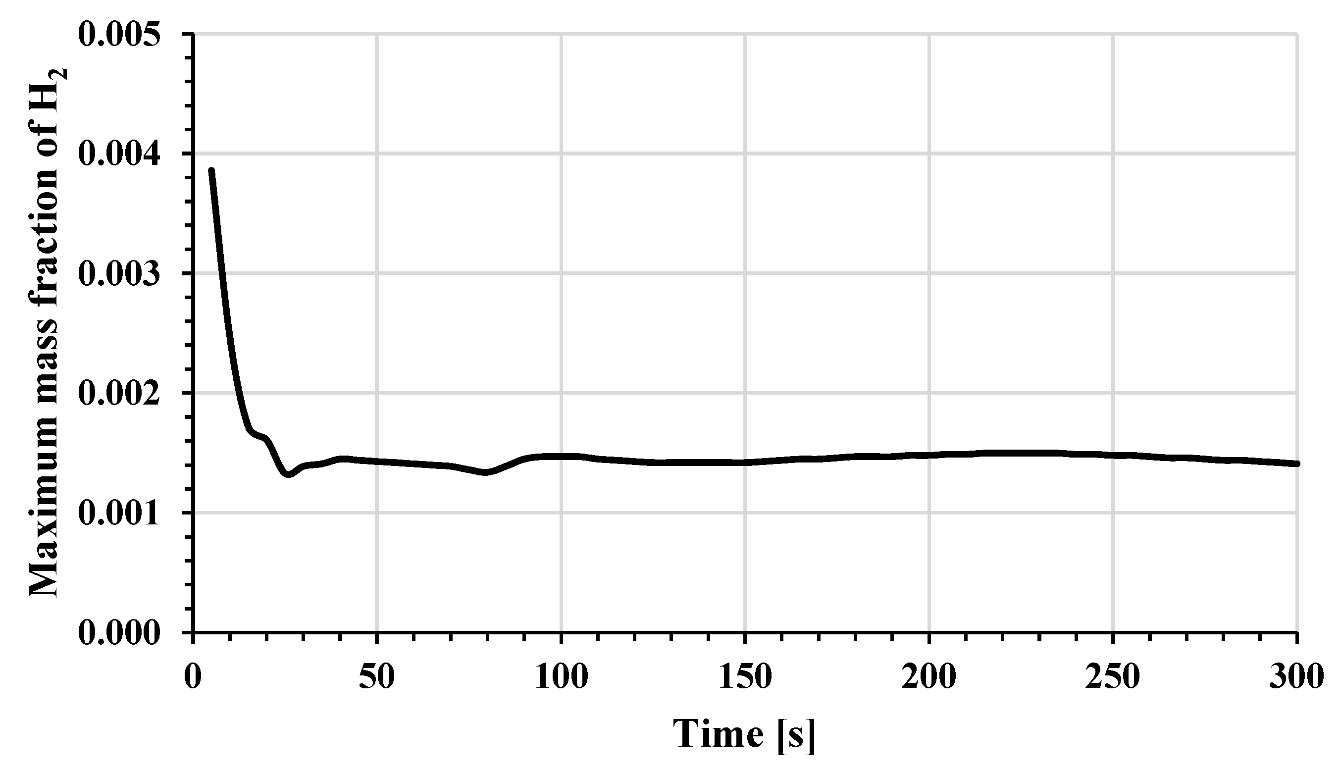
For the maximum mass fraction of H2, we can see a sharp decrease in the values at the early stages (up to 25 s), followed by a period where the values are kept almost constant, as can be seen in Figure 5.
The sharp decrease in the mass fraction of H2 could be potentially related to the consumption of hydrogen during the reverse water–gas shift reaction (RWGS) [Equation (6)]. This reaction consumes hydrogen to produce water. The stabilization of the mass fraction (at 25 s) could indicate that an equilibrium is established in the water–gas shift reaction (WGS) [Equation (6)]. Once the equilibrium is reached, it is expected that the mass fraction of the reactants and products will remain stable.
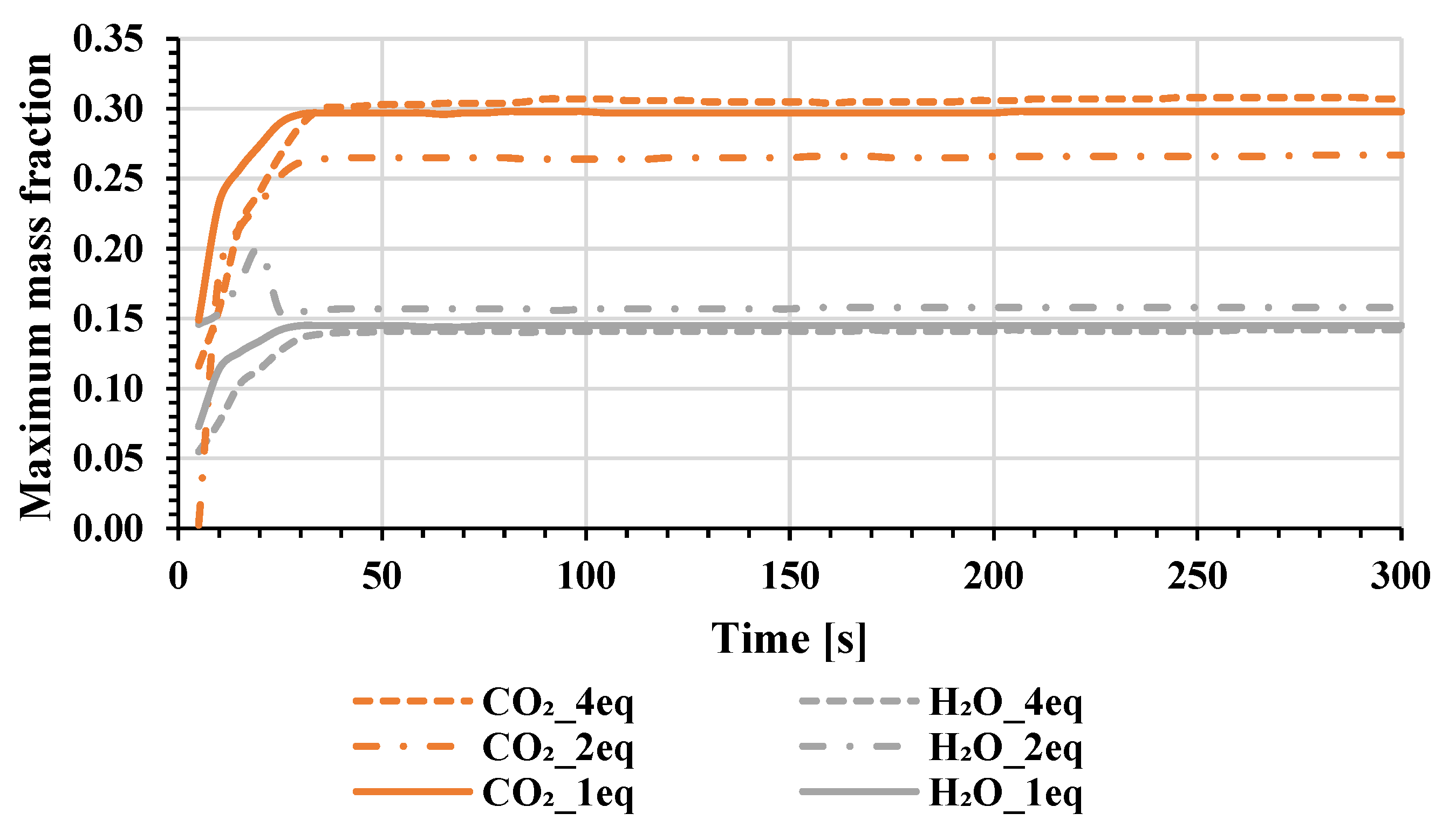
In Figure 6, we can see the maximum mass fraction variation of CO2 and H2O for one-step, two-step, and four-step reactions. It is possible to see a similar behavior for the CO2 mass fraction for the three reactions (one-step, two-step, and four-step). For the one-step and four-step reactions, the values obtained are very close, and the difference between the values obtained at 300 s is 2.9%. The values obtained for the two-step reaction are not so close to the ones obtained for the one-step and four-step reactions; the difference between them is 10.4% at 300 s when we compare the two-step reaction with the one-step reaction. The behavior of the H2O is also similar in the three cases; however, there is a small variation at the start of the two-step reaction when compared with the other two cases. We can see that the values for one-step and four-step reactions are very close, just like for the CO2, and at 300 s, the difference in the value obtained for these two cases is 2.1%. The values obtained for the two-step reaction are slightly different when compared with the other two cases, and at 300 s, the difference is 8.9% between the values obtained for the two-step and one-step reactions.
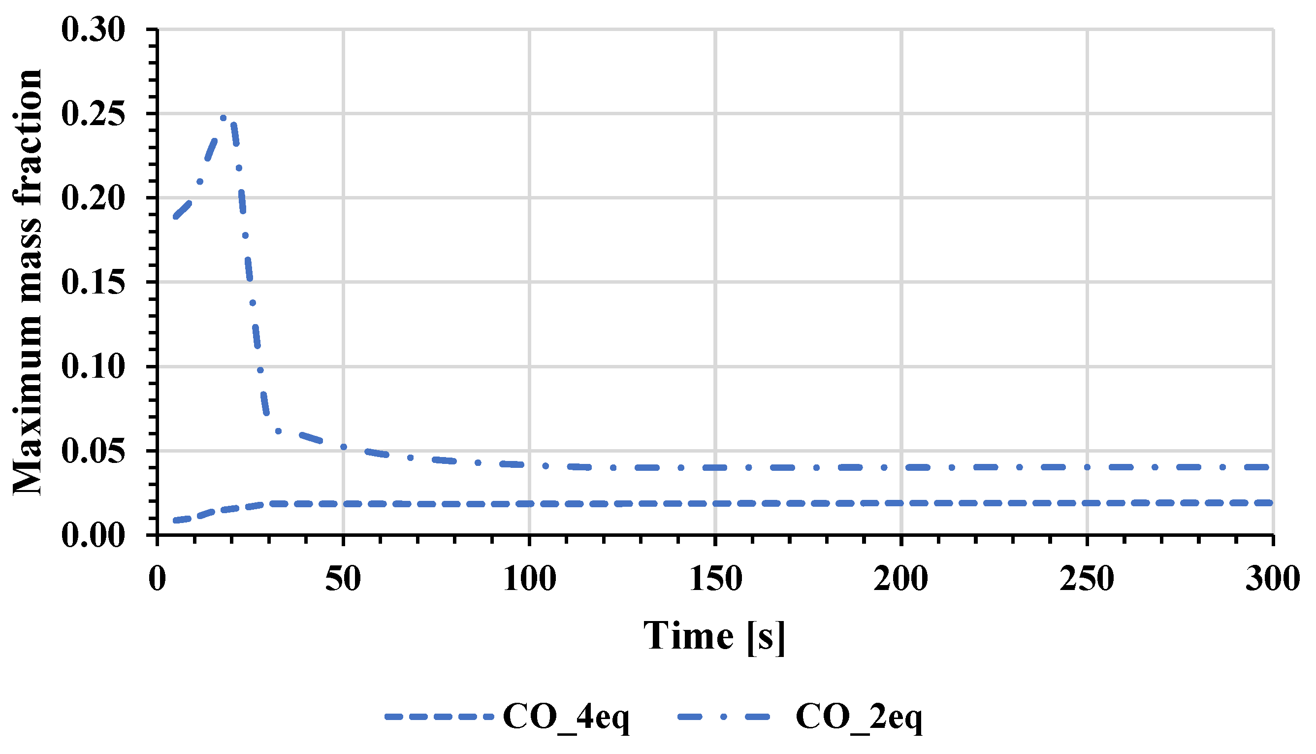
Figure 7 shows the temporal variation of the maximum mass fraction for two-step and four-step reactions. Two different behaviors can be observed since, for the two-step reaction, the mass fraction of CO increases initially and then decreases until it becomes constant (120 s), but for a four-step reaction, initially, there is an increase in the values of mass fraction until they become constant (30 s). At 300 s, the difference between the mass fraction of CO obtained from the four-step and two-step reactions is 52.7%.
Figure 8, Figure 9 and Figure 10 show the variation of the maximum values of temperature, velocity, and turbulent viscosity ratio over time. The three properties mentioned present similar qualitative behavior over time. The temperature increases initially for all three reactions (one-step, two-step, and four-step), and at 300 s presents higher values of temperature for the four-step reaction and lower values for the one-step reaction. The differences in the temperature for the three cases were already expected because, as explained by Yin et al. [12], the molecular dissociation for this type of problem, where the air is used as a reagent, is not expected to have a significant impact on the flame temperature, and typically, the difference in the values can range at most between 200 and 300 K in real flames.
For velocity in Figure 9, we see an initial increase for all three cases, followed by a decrease in the values. After 300 s, we can see that higher velocities are obtained for the one-step equation, and lower velocities are obtained for the two-step reaction. For the turbulence viscosity ratio, Figure 10 also shows an increase in the values at the early stages, followed by a decrease in the values. After 300 s, it is possible to see that the values are close for all cases, but the highest value is obtained for the one-step mechanism, and the lowest value is obtained for the four-step mechanism.
At 300 s, for the temperature, a difference of 3.9% between the values obtained for four-step and two-step reaction mechanisms was obtained, as well as a difference of 3.5% between the two-step and one-step reaction mechanisms. For the velocity, a difference of 2.3% and a difference of 13.3% were obtained between the utilization of four-step and two-step reactions and for the use of one-step and four-step reactions, respectively. For the turbulent viscosity ratio, differences of 10.2% and 4.4% were obtained between the use of four-step and two-step reactions and for the use of one-step and two-step reactions, respectively.
Based on our experience with previous work, e.g., [24,25,26], the numerical error of the present results is approximately 5%. Therefore, the differences observed in the temperature values for the three mechanisms may not be statistically significant. However, the difference between the one-step and four-step reactions is significant, with a 13.3% difference in velocity. Additionally, there is a significant difference of 10.2% in turbulence between the two-step and four-step reactions. These differences highlight the importance of selecting the appropriate mechanism for accurately predicting the temperature, velocity, and turbulence of the system.
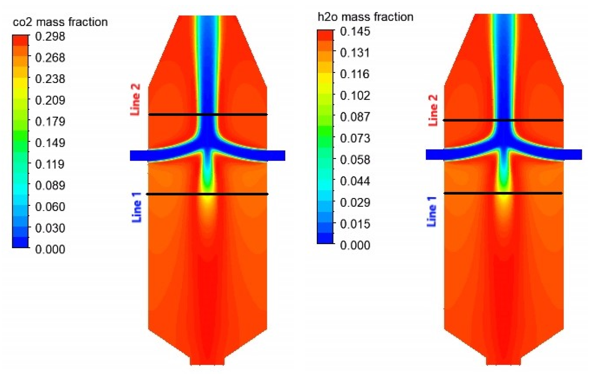
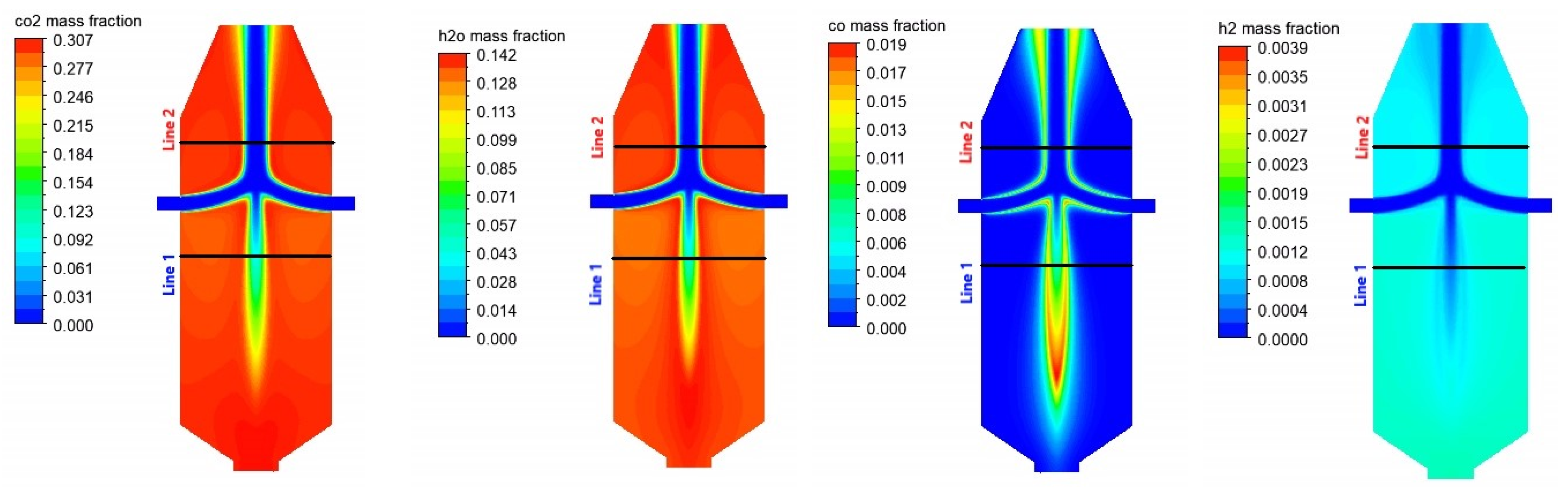
For a more localized analysis of the behavior of the produced species (CO, CO2, H2O, and H2), Figure 11, Figure 12 and Figure 13 show the contour of the product species for the three mechanisms (one-step, two-step, and four-step reactions). Two lines were also drawn on the gasifier to analyze the variation of these species over time in the upper and lower parts of the gasifier.
Based on the previous figures (Figure 11, Figure 12 and Figure 13), it is possible to identify a similar contour between two products from the one-step mechanism at 300 s (CO2 and H2O). This indicates that areas with a greater mass fraction of CO2 will also contain a greater mass fraction of H2O, and vice versa.
For a two-step mechanism and four-step mechanism, the contours of CO and H2 show that the amount of mass fraction present in the gasifier is low. This was already expected since the two-step mechanism favors the creation of CO2 by consuming CO (Equation (3)), and the same happens in the four-step mechanism, where H2 is being converted into H2O (Equations (6) and (7)).
Figure 14 shows the variation of the average mass fraction of CO2 and H2O in the two lines for a one-step reaction mechanism over time. For the initial time steps, there is an increase in the values of mass fraction of CO2 and H2O in both lines, and for the final time steps, the values obtained are constant over time. A similar behavior is observed for both lines, and the average mass fraction values for line 1 are higher than the values for line 2 in almost every time step.
Figure 15 shows the variation of the average mass fraction of CO2, H2O, and CO in the two lines for a two-step reaction mechanism over time. As seen in Figure 12, we can identify a similar behavior of the species over time for the two lines, and the average mass fraction values for line 1 are higher when compared with the values for line 2 in almost every time step.
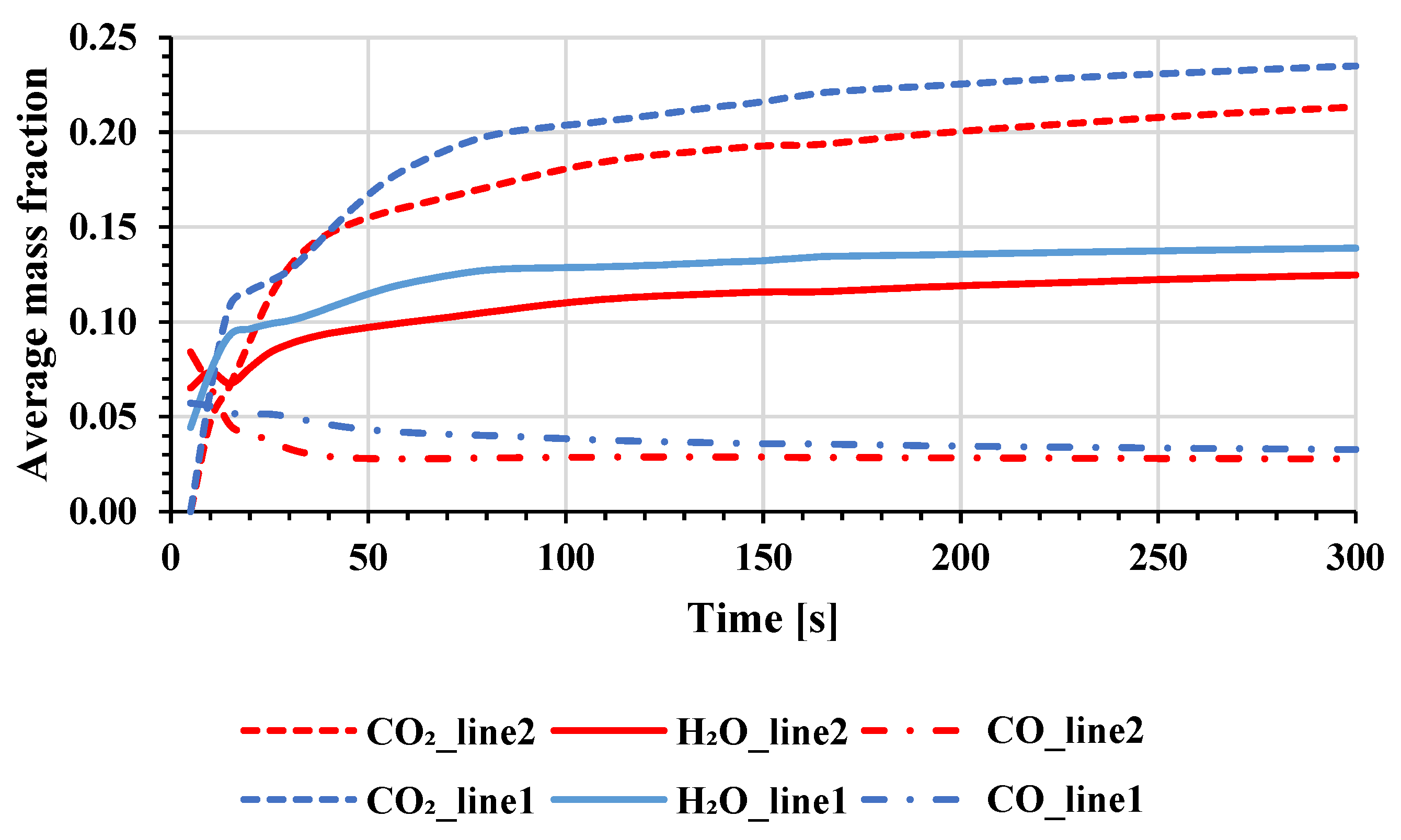
Figure 16 and Figure 17 show the variation of the average mass fraction of CO2, H2O, CO, and H2, respectively, in the two lines for a four-step reaction mechanism over time. Like the cases for one-step and two-step reactions, it is possible to observe the same behavior of the species for the two lines, and the average values are higher for line 1 in almost every time step.
4. Conclusions
For a transitory regime, the behavior of the combustion inside a gasifier was investigated. The results show that the three mechanisms—one-step, two-step, and four-step—had the same qualitative behavior over time for the temperature, velocity, and turbulence fields.
It was observed that the four-step mechanism presents the highest value of temperature at 300 s but has the lowest turbulence. The opposite occurs for the one-step mechanism.
Taking into account the typical numerical uncertainty of the results, which is around 5%, the differences in temperature between the three mechanisms may not be statistically significant. However, it was observed that the differences in the velocity and turbulence fields are more significant.
Furthermore, the difference between the mass fraction of the products between the one-step and four-step mechanisms was also found to not be statistically significant, with differences of 2.9% and 2.1% for the mass fraction of CO2 and H2O, respectively. However, these differences are more significant when compared to the two-step mechanism.
The mass fraction of CO was shown to behave differently under two mechanisms. For the four-step reaction mechanism, values were seen to grow over time, whereas, for the two-step reaction mechanism, values were seen to increase initially before declining until 120 s, at which point they remained nearly constant. This could be explained by the reactions. For the two-step reaction, CO is being consumed to generate CO2; however, for the four-step reaction, the presence of the two extra reactions leads to the formation of CO and H2O, which could explain the initial decrease in H2 and an increase in CO.
The average mass fraction of the species values obtained for the two lines (line 1 and line 2) indicate that higher values are obtained for line 1 for all species, which may imply that a higher mass fraction of the species values can be obtained in the lower half of the gasifier and lower values in the top half of the gasifier.
On the other hand, it is crucial to consider the constraints inherent to two-dimensional simulations, which cannot capture the three-dimensional turbulent effects. This limitation can influence the combustion rate and the development of reaction products. However, 2D simulations facilitate sensitivity analysis, allowing the evaluation of the effects of various parameters on combustion and providing an overview of the evolution of temperature and concentrations of chemical species. By employing 3D simulations of combustion in a gasifier, we aim to acquire more realistic predictions, as the transition to a 3D model provides a more comprehensive representation of real-world phenomena, revealing better understanding through increased complexity, although it can potentially modify system dynamics, such as fluid flow patterns.
Author Contributions
Conceptualization, F.N., A.A.S. and A.R.; methodology, F.N. and A.A.S.; software, F.N. and A.A.S.; validation, A.A.S. and A.R.; investigation, F.N.; writing—original draft preparation, F.N.; writing—review and editing, F.N., A.A.S. and A.R.; supervision, A.A.S. and A.R.; funding acquisition, A.R. All authors have read and agreed to the published version of the manuscript.
Funding
This work is supported by national funds from the FCT–Portuguese Foundation for Science and Technology under project PCIF/GVB/0169/2019.
Institutional Review Board Statement
Not applicable.
Informed Consent Statement
Not applicable.
Data Availability Statement
The original contributions presented in the study are included in the article, further inquiries can be directed to the corresponding author.
Conflicts of Interest
The authors declare that they have no known competing financial interests or personal relationships that could have appeared to influence the work reported in this paper.
References
- Eren, B.; Taspinar, N.; Gokmenoglu, K. The impact of financial development and economic growth on renewable energy consumption: Empirical analysis of India. Sci. Total Environ. 2019, 663, 189–197. [Google Scholar] [CrossRef]
- Charfeddine, L.; Kahia, M. Impact of renewable energy consumption and financial development on CO2 emissions and economic growth in the MENA region: A panel vector autoregressive (PVAR) analysis. Renew. Energ. 2019, 139, 198–213. [Google Scholar] [CrossRef]
- Al-Mulali, U.; Ozturk, I.; Solarin, S. Investigating the environmental Kuznets curve hypothesis in seven regions: The role of renewable energy. Ecol. Indic. 2016, 67, 267–282. [Google Scholar] [CrossRef]
- Khodaei, H.; Guzzomi, F.; Patiño, D.; Rashidian, B.; Yeoh, G. Air staging strategies in biomass combustion-gaseous and particulate emission reduction potentials. Fuel Process. Technol. 2017, 157, 29–41. [Google Scholar] [CrossRef]
- Yolcan, O. World energy outlook and state of renewable energy: 10-Year evaluation. Innov. Green Dev. 2023, 2, 100070. [Google Scholar] [CrossRef]
- Marangwanda, G.; Madyira, D.; Babarinde, T. Combustion models for biomass: A review. Energy Rep. 2020, 6, 664–672. [Google Scholar] [CrossRef]
- Jenkins, B.; Baxter, L.; Miler, T., Jr.; Miles, T. Combustion proprieties of biomass. Fuel Process. Technol. 1998, 54, 17–46. [Google Scholar] [CrossRef]
- Khan, A.; de Jong, W.; Jansens, P.; Spliethoff, H. Biomass combustion in fluidized bed boilers: Potential problems and remedies. Fuel Process. Technol. 2009, 90, 21–50. [Google Scholar] [CrossRef]
- Garba, A. Biotechnolgical Applications of Biomass; Intechopen: London, UK, 2021. [Google Scholar]
- Tabet, F.; Gökalp, I. Review on CFD based models for co-firing coal and biomass. Renew. Sust. Energ. Rev. 2015, 51, 1101–1114. [Google Scholar] [CrossRef]
- Shiehnejadhesar, A.; Scharler, R.; Mehrabian, R.; Obernberger, I. Development and validation of CFD models for gas phase reactions in biomass grate furnaces considering gas streak formation above the packed bed. Fuel Process. Technol. 2015, 139, 142–158. [Google Scholar] [CrossRef]
- Brown, R.C. (Ed.) Thermochemical Processing of Biomass: Conversion into Fuels, Chemicals, and Power, 2nd ed.; Jonh Wiley & Sons: Hoboken, NJ, USA, 2019. [Google Scholar]
- Jones, W.; Lindstedt, R. Global Reaction Schemes for Hydrocarbon Combustion. Combust. Flame 1988, 73, 233–249. [Google Scholar] [CrossRef]
- Yin, C.; Rosendahl, L.; Kær, S. Chemistry and radiation in oxy-fuel combustion: A computational fluid dynamics modeling study. Fuel 2011, 90, 2519–2529. [Google Scholar] [CrossRef]
- Marinov, N.; Westbrook, C.; Pitz, W. Detailed and global chemical kinetics model for hydrogen. In Proceedings of the 8th International Symposium on Transport Proprieties, San Francisco, CA, USA, 16–20 July 1995. [Google Scholar]
- Yin, C.; Rosendahl, L.; Kær, S. Towards a better understanding of biomass suspension co-firing impacts via investigating a coal flame and a biomass flame in a swirl-stabilized burner flow reactor under same conditions. Fuel Process. Technol. 2012, 98, 65–73. [Google Scholar] [CrossRef]
- Álvarez, L.; Yin, C.; Riaza, J.; Pevida, C.; Pis, J.; Rubiera, F. Biomass co-firing under oxy-fuel conditions: A computational fluid dynamics modelling study and experimental validation. Fuel Process. Technol. 2014, 120, 22–33. [Google Scholar] [CrossRef]
- Medina, P.; Núñez, J.; Ruiz-García, V.; Beltrán, A. Experimental and numerical comparison of CO2 mass flow rate emissions, combustion and thermal performance for a biomass plancha-type cookstove. Energy Sustain. Dev. 2021, 63, 153–159. [Google Scholar] [CrossRef]
- Ramezani, M.; Legg, M.J.; Haghighat, A.; Li, Z.; Vigil, R.D.; Olsen, M.G. Experimental investigation of the effect of ethyl alcohol surfactant on oxygen mass transfer and bubble size distribution in an air-water multiphase Taylor-Couette vortex bioreactor. Chem. Eng. J. 2017, 319, 288–296. [Google Scholar] [CrossRef]
- Liu, Y.; Liu, J.T.; Li, X.L. Large eddy simulation of particle hydrodynamic characteristics in a dense gas-particle bubbling fluidized bed. Powder Technol. 2024, 433, 119285. [Google Scholar] [CrossRef]
- Li, Q.; Xu, P.; Li, L.; Xu, W.; Tan, D. Investigation on the lubrication heat transfer mechanism of the multilevel gearbox by the lattice boltzmann method. Processes 2024, 12, 381. [Google Scholar] [CrossRef]
- Ge, Z.; Zheng, G. Fluid-Solid mixing transfer mechanism and flow patterns of the double-layered impeller stirring tank by the CFD-DEM method. Energies 2024, 17, 1513. [Google Scholar] [CrossRef]
- Li, L.; Xu, W.; Tan, Y.; Yang, Y.; Yang, J.; Tan, D. Fluid-induced vibration eveolution mechanism of multiphase free sink vortex and the muti-source vibration sensing method. Mech. Syst. Signal Process. 2023, 189, 110058. [Google Scholar] [CrossRef]
- Morais, A.; Soares, A.; Rouboa, A. A numerical study of the urban wood waste gasification. Energy Rep. 2022, 8, 1053–1062. [Google Scholar] [CrossRef]
- Ismail, T.; Ramos, A.; El-Salam, M.; Monteiro, E.; Rouboa, A. Plasma fixed bed gasification using an Eulerian model. Int. J. Hydrogen Energy 2019, 44, 28668–28684. [Google Scholar] [CrossRef]
- Ismail, T.; Ramos, A.; El-Salam, M.; Monteiro, E.; Rouboa, A. An Eulerian model for forest residues gasification in a plasma gasifier. Energy 2019, 182, 1069–1083. [Google Scholar] [CrossRef]
- Westbrook, C.; Dryer, F. Simplified Reaction Mechanisms for the Oxidation of Hydrocarbon Fuels in Flames. Combust. Sci. Technol. 1981, 27, 31–43. [Google Scholar] [CrossRef]
- Souza-Santos, M. Comprehensive modelling and simulation of fluidized bed boilers and gasifiers. Fuel 1989, 68, 1507–1521. [Google Scholar] [CrossRef]
- Arastoopour, H. Numerical simulation and experimental analysis of gas/solid flow systems: 1999 Fluor-Daniel Plenary lecture. Powder Technol. 2001, 119, 59–67. [Google Scholar] [CrossRef]
- ANSYS. Available online: https://www.afs.enea.it/project/neptunius/docs/fluent/html/th/node58.htm (accessed on 15 June 2023).
Figure 1.
Two-dimensional geometry of the gasifier.

Figure 2.
Evolution of maximum mass fraction CO2 and H2O over time for 1-step reaction.

Figure 3.
Evolution of maximum mass fraction of the products over time for 2-step reaction.

Figure 4.
Evolution of maximum mass fraction of the products over time for 4-step reaction.

Figure 5.
Maximum mass fraction values variation of H2 over time.

Figure 6.
Maximum mass fraction over time of H2O and CO2 for 1-step, 2-step, and 4-step reactions.

Figure 7.
Maximum mass fraction over time of CO for 2-step and 4-step reactions.

Figure 8.
Maximum values of temperature variation over time for 1-step, 2-step, and 4-step reactions.
Figure 8.
Maximum values of temperature variation over time for 1-step, 2-step, and 4-step reactions.

Figure 9.
Maximum values of velocity variation over time for 1-step, 2-step, and 4-step reactions.

Figure 10.
Maximum values of turbulent viscosity ratio variation over time for 1-step, 2-step, and 4-step reactions.
Figure 10.
Maximum values of turbulent viscosity ratio variation over time for 1-step, 2-step, and 4-step reactions.

Figure 11.
Contours of mass fraction of CO2 and H2O for 1-step mechanism at 300 s.

Figure 12.
Contours of mass fraction of CO2, H2O, and CO for 2-step mechanism at 300 s.

Figure 13.
Contours of mass fraction of CO2, H2O, CO, and H2 for 4-step mechanism at 300 s.

Figure 14.
Variation of the average mass fraction of CO2 and H2O in the two lines for a 1-step reaction mechanism over time.
Figure 14.
Variation of the average mass fraction of CO2 and H2O in the two lines for a 1-step reaction mechanism over time.

Figure 15.
Average mass fraction of CO2, H2O, and CO in the two lines for a 2-step reaction mechanism over time.
Figure 15.
Average mass fraction of CO2, H2O, and CO in the two lines for a 2-step reaction mechanism over time.

Figure 16.
Average mass fraction of CO2, H2O, and CO in the two lines for a 4-step reaction mechanism over time.
Figure 16.
Average mass fraction of CO2, H2O, and CO in the two lines for a 4-step reaction mechanism over time.

Figure 17.
Average mass fraction of H2 in the two lines for a 4-step reaction mechanism over time.

Disclaimer/Publisher’s Note: The statements, opinions and data contained in all publications are solely those of the individual author(s) and contributor(s) and not of MDPI and/or the editor(s). MDPI and/or the editor(s) disclaim responsibility for any injury to people or property resulting from any ideas, methods, instructions or products referred to in the content. |
© 2024 by the authors. Licensee MDPI, Basel, Switzerland. This article is an open access article distributed under the terms and conditions of the Creative Commons Attribution (CC BY) license (https://creativecommons.org/licenses/by/4.0/).
Share and Cite
MDPI and ACS Style
Neves, F.; Soares, A.A.; Rouboa, A. A Comparison of Different Biomass Combustion Mechanisms in the Transient State. Energies 2024, 17, 2092. https://0-doi-org.brum.beds.ac.uk/10.3390/en17092092
AMA Style
Neves F, Soares AA, Rouboa A. A Comparison of Different Biomass Combustion Mechanisms in the Transient State. Energies. 2024; 17(9):2092. https://0-doi-org.brum.beds.ac.uk/10.3390/en17092092
Chicago/Turabian StyleNeves, Filipe, Armando A. Soares, and Abel Rouboa. 2024. "A Comparison of Different Biomass Combustion Mechanisms in the Transient State" Energies 17, no. 9: 2092. https://0-doi-org.brum.beds.ac.uk/10.3390/en17092092
Note that from the first issue of 2016, this journal uses article numbers instead of page numbers. See further details here.