An Improved Analytical Thermal Rating Method for Cable Joints

Abstract

To improve the utilization rate of cable lines while retaining sufficient security, the accurate thermal assessment of cable is significant for cable operation condition evaluation. The thermal rating for a cable joint, which is regarded as a hot spot of cable lines, is not covered by the scope of IEC 60287. While the existing publications for cable joint thermal evaluation also have some limitations. In this paper, the quasi-three-dimensional thermal model of the cable joint was established and the iterative solution method for the model is presented. Based on the model, an improved thermal rating method for the cable joint was proposed, which was implemented with monitored surface temperature and load data. The improved method was verified by the finite element method and the results showed an error of less than 5%. The superiority of the improved method was conducted by the comparison between the previously published method and the improved method. The improved method showed a better accuracy than the previously published method. The proposed method in this paper can be complementary to the IEC method, and is easy to use for the operating evaluation of cable joints in the field with the on-line condition monitoring technology.

1. Introduction

Due to the mismatch between the increasing rate of electricity demand and that of the new cable lines, the transmission capacity requirement of existing cable lines is intensifying gradually [1,2,3]. To alleviate this situation, it is important to fully develop the ampacity of existing cable lines. The thermal rating of cable is decided by the cable conductor temperature [4,5]. Thus, the thermal calculation of cable is the key to accurately evaluating the ampacity of cable lines.

Currently, the steady-state thermal evaluation of cable line is generally carried out according to the IEC 60287 method [6]. However, the IEC 60287 method is only used for the cable, while the cable joint is not included. For the cable joint with a large volume, thick main insulation, and poor heat dissipation ability, it often becomes the hot spot in the cable line [7,8]. In the case of low load operation, it is feasible to evaluate the safety of the whole line by using the temperature of the cable. While, in the case of high load operation, although the calculated cable temperature is still within the safe operating range, the insulation temperature of cable joints may be higher than the maximum permissible temperature. Overheated operation of cable joints may lead to deterioration of insulation materials, causing partial discharge, breakdown and explosion, fire, and other serious power accidents [9,10,11].

As supplements to IEC 60287, different thermal evaluation methods for cable joints have been proposed. These methods can be classified into two categories (i.e., numerical methods and analytical methods). The numerical methods (including finite element method, finite difference method, and boundary element method, etc.) can be used to solve and calculate the temperature distribution of cable joints through computer software [12,13,14,15,16].

In [13], Wang P et al. (2017) establish a two-dimensional axial model of a cable joint. The accuracy of the model was verified by field experiments. Using the model, the hot spots of internal insulation in the cable joint were pointed out, and the influence of the convective heat transfer coefficient and ambient temperature on the ampacity of the cable joint was analyzed. In [15], the two-dimensional simulation model and the three-dimensional simulation model of the cable joint were built by Pilgrim, J.A et al (2009), respectively. Then, the difference of the calculation accuracy when the two models were applied to solve the temperature distribution of the cable joint was demonstrated. In [16], a three-dimensional electromagnetic-thermal coupling model of the cable joint was proposed and the influence of the contact resistance on the hot spot temperature of the cable joint was explored by Yang, F et al. (2016). The mentioned numerical methods have the advantage of high calculation accuracy. However, the modelling is complex and slow to calculate the temperature of the cable joint compared with the analytical methods, which makes the application of numerical methods limited.

The analytical methods are used to establish the thermal model of the cable joint and solve the temperature distribution based on the electrothermal analogy theory. In [17], Ruan, J.-J et al (2016) construct a simplified three-dimensional thermal model of the cable joint. Based on the model, the conductor temperature of the cable was obtained from the surface temperature of the cable along the radial direction, then the conductor temperature distribution of the cable joint was solved by the axial inversion. However, for the axial inversion calculation of the conductor temperature, the expressions of temperature solution under different loads need to be re-fitted according to the temperature of the key points, which makes this method less practical. In [8,18], Gouda, O et al. (2016) and Aziz, M.M.A et al. (1980) present the electrothermal analytic model, which considered the axial heat transfer for calculating the conductor temperature distribution of cable joints. However, the solution of this model depends on the setting of boundary conditions, which means unreasonable boundary conditions will result in the inaccuracy of the model. Based on the three-dimensional heat network model of cable joints, Bragatto, T et al. (2019, 2017) propose a thermal calculation method for the cable joint that comprehensively considered laying conditions, weather conditions, and other influencing factors in the literature [19,20]. This method can accurately evaluate the nonlinear thermal behavior of cable joints. But it is difficult to solve the model due to many factors affecting the thermal evaluation of cable joints, making it hard to combine it with the existing on-line temperature monitoring system of cable joints.

In this paper, a quasi-three-dimensional thermal model of cable joints was established and an iterative method for solving the model was provided. In practical application, the surface temperature of cable joints can be obtained by thermal imaging technology as input quantity, and the conductor temperature can be solved quickly.

Based on the model, an improved steady-state thermal evaluation method for cable joints was proposed, taking the monitored surface temperature and the line load as inputs. The accuracy and superiority of the improved method were verified by the finite element analysis (i.e., FEA) method. The results show that the proposed improved method presents a satisfactory performance on cable joint thermal rating. The improved method proposed in this paper can be easily incorporated into the existing temperature on-line monitoring system of cable lines, and the conductor temperature distribution of the cable joint can be solved based on the on-line monitoring data, so as to realize the accurate evaluation of the operating state of cable joints.

2. Review of Traditional Electrothermal Analytic Method for Cable Joints

Compared with the cable, the cable joint has a thicker insulation, larger volume, and poor heat dissipation capability, resulting in a higher conductor temperature of the cable joint than that of the adjacent cable. According to the second law of thermodynamics, heat will be transferred spontaneously from a high-temperature object to a low-temperature object. Thus, part of the internal heat from the cable joint will be transferred along the copper conductor with high thermal conductivity to the cable with lower temperature, causing the conductor temperature of the cable to rise. Meanwhile, there is a temperature difference between the surface of the cable joint and the environment, so part of the internal heat will be exchanged with the surrounding environment. As a result, the heat dissipation process of the cable joint is actually a three-dimensional problem.

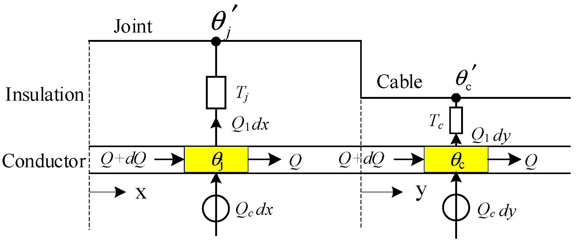
To address the three-dimensional heat transfer problem of the cable joint, the traditional electrothermal analytic method for calculating the conductor temperature of the cable joint, considering the influence of axial heat transfer, was first proposed in [18] and further developed in [8], which was named the traditional electrothermal analysis (i.e., TEA) method in the following. In the TEA method, it was assumed that the cable and the cable joint were isotropic along the radius direction, and then the three-dimensional thermal conductivity problem of the cable joint and cable can be simplified into a two-dimensional thermal conductivity problem. In the meantime, the influence of some asymmetric structure in the cable joint on the temperature distribution was ignored. Setting the center of the cable joint as the initial point, a quarter-element thermal model of the cable joint and adjacent cable was established, as shown in Figure 1.

In Figure 1, θ_j is the conductor temperature of the cable joint, θ_c is the conductor temperature of the cable, θ_j′ is the surface temperature of the cable joint, θ_c′ is the surface temperature of the cable, T_j is the total radial thermal resistance of the cable joint, T_c is the total radial thermal resistance of the cable, Q is the axial heat flux in the conductor, Q_c is the conductor joule loss, and Q₁ is the radial heat flux transferred from the conductor to the environment. The expressions are respectively as follows,

$$Q=\frac{A}{\rho }\frac{d\theta }{dx}$$

(1)

$$Q_c=I^2{R}_{20}[1+\alpha (\theta -20)]$$

(2)

$$Q_1=\frac{\theta -{\theta }^{\prime }}{T_t}$$

(3)

where, ρ is the thermal resistivity of the conductor, A is the conductor cross-sectional area, I is the cable load, R₂₀ is the resistance of the conductor at 20 °C, and α is the temperature coefficient of the resistance of the conductor. Based on the thermoelectric analogy method, the following heat balance equation can be set up.

$$\frac{dQ}{dx}=Q_1-Q_c$$

(4)

For the cable joint and cable, the radial thermal resistance of each layer of the structure can be calculated according to the thick-wall model of a cylinder. According to the IEC 60287 method, the total radial thermal resistance (T_t) per unit length of cable joint and body can be calculated as follows [6],

$$T_t={\displaystyle \sum _{i=1}^n\frac{1}{2\pi {\lambda }_i}\ln (\frac{d_{i+1}}{d_i})}$$

(5)

where λ_i is the thermal conductivity of the materials in each layer, d_i+1 and d_i are the outer and inner diameters of each layer, respectively.

The second-order inhomogeneous differential equation of the conductor temperature can be obtained by combining Equations (1)~(4), then the result is shown in (6).

$$\left\{\begin{array}{l}-a_2\frac{d^2\theta }{d{x}^2}+a_0\theta =M\\ a_2=A{T}_t/\rho \\ a_0=\left(1-\alpha I^2{R}_{20}{T}_t\right)\\ M={\theta }^{\prime }+\left(1-20\alpha \right)I^2{R}_{20}{T}_t\end{array}\right.$$

(6)

In the TEA method, because the heat flux along the axial direction mainly exists in the materials with high thermal conductivity [7] and the copper shell has a smaller temperature gradient as it is too far away from the heat source, it is assumed that there is no axial heat flux existing between the central element and the adjacent elements of the cable joint except for the conductor, neither between the cable terminal element and its adjacent elements. Also, the temperature and the axial heat flux of the adjacent elements at the interface between the cable joint and cable are the same. L_j is defined as half of the total length of the cable joint, and the following four boundary conditions are obtained:

$${\left.\frac{d{\theta }_j}{dx}\right|}_{x=0}=0$$

(7)

$${\left.{\theta }_j\right|}_{(x=L_j)}={\left.{\theta }_c\right|}_{(y=0)}$$

(8)

$${\left.\frac{d{\theta }_j}{dx}\right|}_{x=L_j}={\left.\frac{d{\theta }_c}{dy}\right|}_{y=o}$$

(9)

$${\left.\frac{d{\theta }_c}{dy}\right|}_{(y=\infty )}=0$$

(10)

Combined with the boundary conditions, the second-order differential equation shown in (6) is solved, and the conductor temperature distribution of the cable joint and adjacent cable is finally obtained as the following expression.

$$\begin{array}{l}{\theta }_j(x)=\frac{M_j}{a_{0j}}+B_j·\cosh (\sqrt{\frac{a_{0j}}{a_{2j}}}·x)\\ {\theta }_c(y)=\frac{M_c}{a_{0c}}-B_j·\sqrt{\frac{a_{0j}{a}_{2c}}{a_{oc}{a}_{2j}}}·\left[\cosh (\sqrt{\frac{a_{0c}}{a_{2c}}}·y)-\sinh (\sqrt{\frac{a_{0c}}{a_{2c}}}·y)\right]\\ B_j=\frac{M_c/a_{0c}-M_j/a_{0j}}{\cosh (\sqrt{a_{0j}/a_{2j}}·L_j)+\sqrt{(a_{0j}{a}_{2c})/(a_{2j}{a}_{0c})}·\sinh (\sqrt{a_{0j}/a_{2j}}·L_j)}\end{array}$$

(11)

The TEA method takes full account of the axial heat flux in the conductor between the cable joint and adjacent cable. It provides a convenient and practical method for the thermal evaluation of the cable joint. However, the calculation accuracy of the TEA method is low, mainly for the following reasons:

(1) The cable joint is simplified to a simple geometric structure. However, the actual cable joint structure is complex, and the radial thickness of each layer at different positions is not consistent. This simplification will lead to an inaccurate calculation of radial thermal resistance.

(2) The value of the axial heat flux between two adjacent elements is determined by the axial temperature difference between the two elements. However, the TEA method assumes that the axial heat fluxing into the element only depends on the conductor temperature of the element. Thus, the unreasonable calculation of axial heat flux will bring error to the calculation result of the conductor temperature.

(3) The TEA method assumes that there is no axial heat flux between the cable joint central element and its adjacent element, which will result in a conductor isothermal region near the center of the cable joint. But in the actual situation, the cable joint is often unable to form a conductor isothermal region near the center due to its length limitation. Thus, the setting of boundary condition (7) will make the calculated result of the hot spot temperature of the cable joint higher.

3. Thermal Finite Element Analysis of Cable Joint

To improve the accuracy of the thermal calculation of the cable joint and provide support for the reliability evaluation of the cable joint operating status, it is necessary to put forward a more accurate thermal rating method for the cable joint. Before that, to better understand the axial heat transfer characteristics of the cable joint, a thermal simulation model of the cable joint was established to calculate the temperature distribution, which can provide the basis for the verification of the subsequent improved thermal rating method for the cable joint.

3.1. Two-Dimensional (2D) Axisymmetric Simulation Model of Cable Joint

The main components of the cable joint are axisymmetric, and the rare asymmetric structures have little influence on the thermal model [13]. In [21], it was pointed out that there is little difference between the joint temperature distribution results calculated by the simplified 2D axisymmetric simulation model and the three-dimensional (3D) simulation model, respectively. Moreover, compared with the 3D simulation model, the simplified 2D axisymmetric simulation model has the advantages of simple modeling process and fast calculation speed. Therefore, in this paper the simplified 2D axisymmetric simulation model of the cable joint was used to realize the thermal calculation of the cable joint.

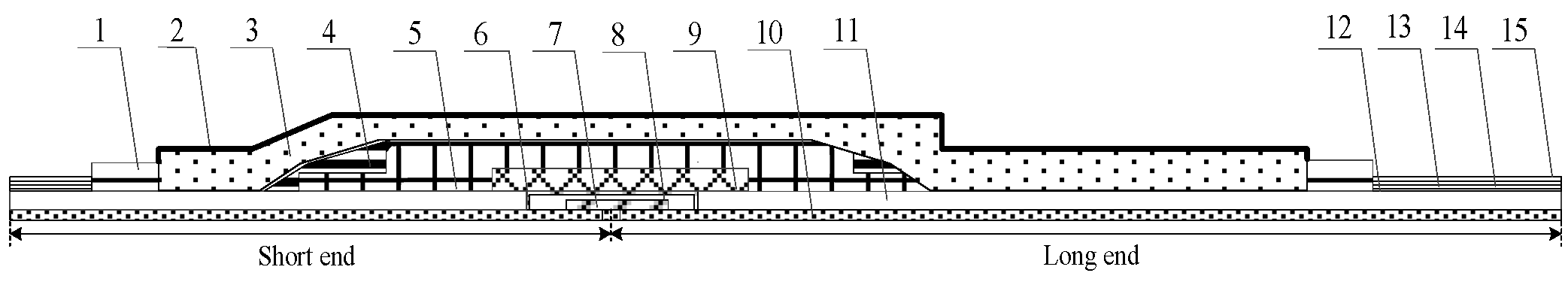
A 110 kV 630 mm² straight-through cable joint laid in the tunnel was selected as the research object, and the established simulation model is presented in Figure 2. The thermal parameters of the cable joint and the cable are shown in

Table 1. Detailed information of the cable joint.

Component	Material	Thermal Conductivity /W·m−1·K−1	Thickness /mm
Conductor tube	Copper	401	15
Air gap	Air	0.023	3
Copper screen tube	Copper	401	7.3
Joint main insulation	Silicone rubber	0.25	/
PVC belt	Polyvinyl chloride	0.1667	2
ab glue sealing	Epoxy resin	0.2	18
Copper shell	Copper	401	3.1

and

Table 2. Parameters of the cable.

Component	Material	Thermal Conductivity /W·m−1·K−1	Diameter /mm
Conductor	Copper	401	30
Conductor shielding	Polyolefin	0.32	33
XLPE insulation	Crosslinked polyethylene	0.286	66
Insulation shielding	Polyolefin	0.32	68
Buffer layer	Polyester fiber	0.1667	75
Air gap	Air	0.023	85.5
Aluminum sheath	Aluminum	238	88.6
Outer sheath	High density polyethylene	0.286	97.6

, respectively. Before installing the cable joint, stripping should be conducted on the cable. After the assembly of the cable joint and cable, the lengths of the left end and right end as centered on the connection tube are inconsistent due to the different stripping lengths. These two parts are respectively marked as the long end and the short end, as shown in Figure 2.

To simplify the model and reduce the difficulty of solving, some simplifications for the geometric structure are assumed [22,23,24].

(1) The grounding columns on the copper shell surface of the cable joint are ignored, and the copper shell is simplified into a flat and smooth cylinder.

(2) The stress cone is merged into the main insulation of the cable joint with similar thermal conductivity.

(3) The corrugated spiral structure of the aluminum sheath is ignored.

To solve the cable joint simulation model, both sides of the model are set as adiabatic boundaries. Considering the complex and changeable tunnel environment in actual operation, it is difficult to directly determine the boundary temperature and the boundary heat flux for the surface of the cable joint and cable. Thus, the convection wall was adopted for the surface of the cable joint and cable [13] and the natural heat transfer coefficient was set at 7.5 W/m·K⁻¹, and the air temperature was set at 19.5 °C. For the cable far away from the cable joint, the influence of the axial heat transfer from the cable joint can be negligible. As a result, the axial temperature difference between the adjacent two cable joint elements can be ignored in the steady state. Only the heat flux transferring along the radial direction needs to be considered. Thus, both radial sections of the cable end were set as the adiabatic surface [14].

3.2. Determination of the Axial Length of the 2D Simulation Model

Compared with the cable, the conductor temperature of the cable joint is significantly higher under the same heat source due to the large volume and poor heat dissipation conditions of the cable joint. Then, some of the heat from the cable joint will be transferred to the adjacent cable along the conductor, raising the conductor temperature of the adjacent cable. However, as the length of the cable increases, the conductor temperature of the cable is less affected by the axial heat flux from the cable joint. To obtain a more accurate thermal assessment of the cable joint, the axial length of the cable in the simulation model should be determined according to the influence range of the axial heat flux. In [13], the method to determine the influence range of axial heat flux of the cable joint has been proposed, which was also adopted for determining the axial length of the simulation model in this paper. Based on this method, the length of the cable at both ends of the model were set to 3 m respectively, and the total length of the simulation model was 8 m.

3.3. Analysis of the Results

For the simulation model, the central location of the connection tube was chosen as the origin of the temperature sampling path, and the long end of the cable joint was set as the positive direction. Then, the detailed temperature distribution sampling paths for the cable joint conductor and surface are shown in Figure 3. The conductor temperature and surface temperature results along the sampling paths under different loads are presented in Figure 4.

For the conductor temperature distribution curves, it can be seen that the peak under different loads all appear at the center of the connection tube. The temperature distribution is characterized by a gradual decrease from the center of the connection tube to both ends, and finally leveling off at the end of the cable. For the surface temperature distribution curves, it can be seen that the surface temperature of the cable joint is lower than that of the cable, showing a concave state. This is because the surface area of the cable joint is larger than the cable, resulting in an increase in radial heat dissipation power, and the radial heat dissipation power is unchanged, so the surface temperature of the cable joint is reduced to maintain the same heat dissipation power. As shown in Figure 4, compared with the surface temperature distribution of the cable, the surface temperature changing gradient of the cable joint along the axial direction is smaller.

4. An Improved Thermal Rating Method for Cable Joint

Combined with the distribution characteristics of the conductor temperature and surface temperature obtained by the simulation model, an improved calculation method for the conductor temperature of the cable joint can be proposed to remedy the deficiency of existing methods.

4.1. A Quasi-3D Axial Thermal Model of Cable Joint

The structure of the cable joint is complex, and the insulation thickness at different positions is not consistent, which will affect the radial thermal resistance. Before establishing the thermal model for more accurate thermal rating, the cable joint was divided into different segments according to the insulation thickness as shown in Figure 5. The center of the connection tube was set as the origin, and the dividing was conducted from the origin to the end of the cable. In Figure 5, A, B, C, and D₁ belong to the short end of the cable joint, while D₂, E, F, and G belong to the long end of the cable joint.

The short end and the long end of the cable joint have a similar structure, but are different in the axial length. Therefore, in this section, the long end of the cable joint was taken as an example to illustrate the establishment process of the quasi-3D thermal model. For the above segmented parts of the cable joint, each segment was further divided into several smaller units along the axial direction by using the idea of infinities. The thermal model in the radial and axial direction were established in reference to [25]. Thus, only the axial heat flux in the conductor was considered in the thermal model. Then, the built quasi-3D thermal model of the long end of the cable joint is shown in Figure 6.

In Figure 6, the radial thermal resistance of each component and the axial thermal resistance between two adjacent conductor units can be calculated by (12) and (13), respectively [6,26],

$$\Delta T_{\mathrm{ys}}=\frac{1}{2\pi {\lambda }_s\Delta z_s}\ln \left(\frac{d_o}{d_i}\right)$$

(12)

$$\Delta T_{xs}=\frac{\Delta z_s}{\pi {\lambda }_c{r}_c^2}$$

(13)

where Δz_s is the unit length, λ_s is the conductivity of different components, λ_c is the thermal conductivity of copper, d_o and d_i is the outer and inner diameters of each component, respectively, and r_c is the radius of the conductor.

4.2. Solution for the Quasi-3D Thermal Model of Cable Joint

For the quasi-3D thermal model of the cable joint as shown in Figure 6, the accuracy of the model highly depended on the number of units. Theoretically, a more accurate temperature calculation result can be obtained with more units. However, the large number of units means a heavy computation and complex solution process. Thus, it is necessary to determine an appropriate number of units to reduce the computation on the premise of ensuring sufficient accuracy of the model.

Based on the thermal simulation results in Section 3, it can be inferred that the surface temperature difference between adjacent cable joint units can be ignored when the cable joint is divided into a sufficient number of units. In [27], based on the assumption that the surface temperatures of adjacent units are the same, the quasi-3D thermal model for the short-conduit cable is simplified by using the Y-Δ transformation method. This simplified method is also feasible for the quasi-3D thermal model of the cable joint in this paper. The simplified quasi-3D thermal model of the long end of the cable joint is shown in Figure 7, which is also applicable for the short end of the cable joint.

In Figure 7, θ_s (s = 1,2…n) is the conductor temperature and θ_s′ is the surface temperature. The model takes the surface temperature of the cable joint, the surface temperature of the cable, and the cable load as the input and takes the conductor temperature as the output. The specific calculation steps are as follows.

(1) In the case of no axial heat flux existing in the cable joint, the conductor temperature is proportional to the radial thermal resistance and the radial heat flux, which can be calculated by (14)

$${\theta }_s^{(1)}=\left\{\begin{array}{ll}{{\theta }_s}^{\prime }+\Delta {Q_{rs}}^{(1)}·\Delta T_{y1}& 1\le s\le j\\ {{\theta }_s}^{\prime }+\Delta {Q_{rs}}^{(1)}·\Delta T_{y2}& j+1\le s\le k\\ {{\theta }_s}^{\prime }+\Delta {Q_{rs}}^{(1)}·\Delta T_{y3}& k+1\le s\le m\\ {{\theta }_s}^{\prime }+\Delta {Q_{rs}}^{(1)}·\Delta T_{y4}& m+1\le s\le n\end{array}\right.$$

(14)

where ΔQ_r is the conductor joule loss, calculated as follows,

$$\Delta {Q_r}^{(1)}=\left\{\begin{array}{ll}{I}^{2}R\left[1+\alpha \left({{\theta }_s}^{(0)}-20\right)\right]·\Delta z_1& 1\le s\le j\\ I^{2}R\left[1+\alpha \left({{\theta }_s}^{(0)}-20\right)\right]·\Delta z_2& j+1\le s\le k\\ I^{2}R\left[1+\alpha \left({{\theta }_s}^{(0)}-20\right)\right]·\Delta z_3& k+1\le s\le m\\ I^{2}R\left[1+\alpha \left({{\theta }_s}^{(0)}-20\right)\right]·\Delta z_4& m+1\le s\le n\end{array}\right.$$

(15)

where Δz₁, Δz₂, Δz₃ and Δz₄ are the unit length of segment D₂, E, F, and G, respectively. In this paper, the initial conductor temperature θ⁽⁰⁾ of each unit was set to 90 °C, then the conductor temperature θ⁽¹⁾ of each unit calculated by (14) was the iterative initial value of the quasi-3D thermal model.

(2) Considering the effect of axial heat flux, the conductor temperature of each unit is determined by the combined action of radial and axial heat flux. For the unit of the connection tube center, there is only the axial heat flux from this unit to the adjacent units, but no axial heat flux to this unit. For the unit at the tail end of the cable, the influence of the axial heat flux on its conductor temperature θ_n can be neglected, then θ_n calculated by the IEC standard can be set as the starting point for the model calculation. The updated conductor temperatures of each unit in the quasi-3D thermal model of the cable joint are calculated as follows.

$${{\theta }_s}^{(i+1)}=\left\{\begin{array}{ll}{{\theta }_s}^{\prime }+\Delta T_{y1}·(\Delta {Q_{rs}}^{(i+1)}-2·\Delta {Q_{xls}}^{(i+1)})& s=1\\ {{\theta }_s}^{\prime }+\Delta T_{y1}·(\Delta {Q_{rs}}^{(i+1)}+\Delta {Q_{x2s}}^{(i)}-\Delta {Q_{xls}}^{(i+1)})& 2\le s\le j\\ {{\theta }_s}^{\prime }+\Delta T_{y2}·(\Delta {Q_{rs}}^{(i+1)}+\Delta {Q_{x2s}}^{(i)}-\Delta {Q_{xls}}^{(i+1)})& j+1\le s\le k\\ {{\theta }_s}^{\prime }+\Delta T_{y3}·(\Delta {Q_{rs}}^{(i+1)}+\Delta {Q_{x2s}}^{(i)}-\Delta {Q_{xls}}^{(i+1)})& k+1\le s\le m\\ {{\theta }_s}^{\prime }+\Delta T_{y4}·(\Delta {Q_{rs}}^{(i+1)}+\Delta {Q_{x2s}}^{(i)}-\Delta {Q_{xls}}^{(i+1)})& m+1\le s\le n-1\end{array}\right.$$

(16)

$$\Delta {Q_r}^{(i+1)}=\left\{\begin{array}{ll}{I}^{2}R\left[1+\alpha \left({{\theta }_s}^{(i)}-20\right)\right]·\Delta z_1& 1\le s\le j\\ I^{2}R\left[1+\alpha \left({{\theta }_s}^{(i)}-20\right)\right]·\Delta z_2& j+1\le s\le k\\ I^{2}R\left[1+\alpha \left({{\theta }_s}^{(i)}-20\right)\right]·\Delta z_3& k+1\le s\le m\\ I^{2}R\left[1+\alpha \left({{\theta }_s}^{(i)}-20\right)\right]·\Delta z_4& m+1\le s\le n-1\end{array}\right.$$

(17)

$$\Delta {Q_{x1}}^{(i+1)}=\left\{\begin{array}{ll}\frac{{\theta }_s^{(i)}-{\theta }_{s-1}^{(i+1)}}{\Delta T_{x1}}& 1\le s\le j-1\\ \frac{{\theta }_s^{(i)}-{\theta }_{s-1}^{(i+1)}}{\Delta T_{xc1}}& s=j\\ \frac{{\theta }_s^{(i)}-{\theta }_{s-1}^{(i+1)}}{\Delta T_{x2}}& j+1\le s\le k-1\\ \frac{{\theta }_s^{(i)}-{\theta }_{s-1}^{(i+1)}}{\Delta T_{xc2}}& s=k\\ \frac{{\theta }_s^{(i)}-{\theta }_{s-1}^{(i+1)}}{\Delta T_{x3}}& k+1\le s\le m-1\\ \frac{{\theta }_s^{(i)}-{\theta }_{s-1}^{(i+1)}}{\Delta T_{xc3}}& s=m\\ \frac{{\theta }_s^{(i)}-{\theta }_{s-1}^{(i+1)}}{\Delta T_{x4}}& m+1\le s\le n-1\end{array}\right.$$

(18)

$$\Delta {Q_{x2}}^{(i)}=\left\{\begin{array}{ll}\frac{{\theta }_{s+1}^{(i)}-{\theta }_s^{(i)}}{\Delta T_{x1}}& 1\le s\le j-1\\ \frac{{\theta }_{s+1}^{(i)}-{\theta }_s^{(i)}}{\Delta T_{xc1}}& s=j\\ \frac{{\theta }_{s+1}^{(i)}-{\theta }_s^{(i)}}{\Delta T_{x2}}& j+1\le s\le k-1\\ \frac{{\theta }_{s+1}^{(i)}-{\theta }_s^{(i)}}{\Delta T_{xc2}}& s=k\\ \frac{{\theta }_{s+1}^{(i)}-{\theta }_s^{(i)}}{\Delta T_{x3}}& k+1\le s\le m-1\\ \frac{{\theta }_{s+1}^{(i)}-{\theta }_s^{(i)}}{\Delta T_{xc3}}& s=m\\ \frac{{\theta }_{s+1}^{(i)}-{\theta }_s^{(i)}}{\Delta T_{x4}}& m+1\le s\le n-1\end{array}\right.$$

(19)

The radial heat flux ΔQ_r in (16) is calculated according to (17). The axial heat flux ΔQ_x1 flowing out of the unit and the axial heat flux ΔQ_x2 flowing into the unit are calculated, respectively, by (18) and (19). When calculating the conductor temperature θ_s⁽ⁱ⁺¹⁾ of the unit s, the conductor temperature of the unit (s + 1) to the unit n was iterated (i + 1) times, while the conductor temperature of the remaining units only was iterated i times. To speed up the convergence rate of the iterative calculation, when calculating the axial heat flux ΔQ_x1 flowing out of the unit s, use the iterative result of the conductor temperature θ_s⁽ⁱ⁾ of the unit s and the iterative result of the conductor temperature θ_s+1⁽ⁱ⁺¹⁾ of the unit (s + 1). When calculating the axial heat flux flowing into the unit s, use the i−th conductor temperature iteration results of unit (s − 1) and units.

In (18) and (19), ΔT_x is the axial thermal resistance between adjacent units within the same segment and ΔT_xc is the axial thermal resistance of different segment connections. The weighted mean of the axial thermal resistance between adjacent units is taken as the value of ΔT_xc, as shown in the following.

$$\Delta T_{xcs}=\left\{\begin{array}{ll}\frac{\Delta z_1+\Delta z_2}{2\pi {\lambda }_c{r}_c^2}& s=1\\ \frac{\Delta z_2+\Delta z_3}{2\pi {\lambda }_c{r}_c^2}& s=2\\ \frac{\Delta z_3+\Delta z_4}{2\pi {\lambda }_c{r}_c^2}& s=3\end{array}\right.$$

(20)

(3) The relevant constraints are applied in the process of model calculation. It can be known from the simulation results that the temperature of the cable joint gradually decreases from the center to both ends, and the axial heat flux is unidirectional. Thus, the axial heat flux should satisfy the constraint condition 1 during the whole calculation, as shown in (21).

$$\Delta Q_x\ge 0$$

(21)

In the initial calculation process, for some units, the inflow axial heat flux may be much greater than the outflow axial heat flux, or the opposite case may occur. It will result that the calculated conductor temperature distribution is contrary to the actual distribution trend. Therefore, the constraint condition 2 is applied to prevent unreasonable results from the calculation of axial heat flux, as shown in (22) and (23),

$$\Delta {Q_{x1}}^{\prime }=\frac{\Delta Q_{x1}}{K_1}$$

(22)

$$\Delta {Q_{x2}}^{\prime }=\frac{\Delta Q_{x2}}{K_1}$$

(23)

where K₁ is the minification, and its value range is K₁ > 1. Based on the axial heat flux calculated by (18) and (19), the axial heat inflow and outflow of the same unit is compared. If ΔQ_x1 > K₁·ΔQ_x2, (22) will be used, and if ΔQ_x2 > K₁·ΔQ_x1, (23) will be used, until meeting the constraint 3 shown in (24). The corrected axial heat flux will be replaced into (16) to calculate the conductor temperature,

$$\left\{\begin{array}{ll}\Delta {Q_{x1}}^{\prime }-\Delta Q_{x2}\le K_2& \left(\mathrm{i}\right)\\ \Delta {Q_{x2}}^{\prime }-\Delta Q_{x1}\le K_2& \left(\mathrm{ii}\right)\end{array}\right.$$

(24)

where K₂ is the constraint coefficient, and its value range is 0 < K₂ < 1. It is to prevent the temperature of the unit conductor from rising or falling sharply in the iteration process. Meanwhile, since the conductor temperature decreases monotonically from the center to both ends, the temperature of the former unit θ_j is always higher than that of the latter unit θ_j+1. Thus, the constraint condition 4 is applied to ensure the monotony of the axial conductor temperature, as shown in (25).

$${\theta }_j^{(i)}\ge {\theta }_{j+1}^{(i)}$$

(25)

In the process of iterative calculation, if the temperature of a unit calculated in this iteration does not meet the constraint condition 4, keep using the previous calculation result, that is, θ_j⁽ⁱ⁾ = θ_j⁽ⁱ⁻¹⁾. After repeated iterations, the temperature of each unit tends to converge. The error between the current iteration calculation result and the last iteration calculation result of the conductor temperature of each unit is selected as the iterative convergence criterion. When the error satisfies (26), the iterative convergence is determined.

$$\left|{\theta }_j^{(i+1)}-{\theta }_j^{(i)}\right|\le 0.1$$

(26)

5. Verification and Discussion

To verify the accuracy of the proposed improved thermal rating method for the cable joint, the straight-through cable joint shown in Figure 2 was taken as the object. Then, for the simplified quasi-3D thermal model of the cable joint, the unit length of segment A, B, C, D₁, D₂, E, F, and G were set to 0.1257 m, 0.075 m, 0.071 m, 0.098 m, 0.098 m, 0.0817 m, 0.0761 m, and 0.1304 m, respectively. The comparisons between the conductor temperature results of the cable joint by using the FEA method and the improved method are presented in Figure 8. The cases of different cable load (1000 A and 1200 A) are respectively shown in Figure 8a,b. The temperature results of the TEA method are also shown in Figure 8 to display the improved accuracy benefit of the improved method. It is worth noting that the improved method is not influenced by the environment, which can be applied to other cable laying manners after minor adjustment.

It is seen from Figure 8 that the temperature distribution curves calculated by three different methods have the same trend, with the temperature decreasing gradually from the center to both ends. The center of the connection tube is the peak temperature of the cable joint, thus the accurate thermal calculation for this point has great significance to the state evaluation of the thermal bottleneck point of the cable line. In Figure 8, it is clarified that the peak conductor temperature of the cable joint calculated by the TEA method has up to 20 °C difference with the simulation result, which shows that the TEA method has a low accuracy in the evaluation of the hotspot temperature of the cable joint. On the other hand, the difference of the peak conductor temperature results of the cable joint between the improved method and the FEA method is within 1 °C, which verifies the accuracy of the improved method.

To highlight the superiority of the improved method compared with the TEA method, the goodness of fit is used to describe the degree of fitting between the temperature distribution curves calculated by different methods and those calculated by the FEA method. The statistic to measure goodness of fit is the determination coefficient R², and its calculation is shown in (27),

$$R^2=1-\frac{{\displaystyle \sum _{i=1}^n{\left(y_i-{\widehat{y}}_i\right)}^2}}{{\displaystyle \sum _{i=1}^n{\left(y_i-\overline{y}\right)}^2}}$$

(27)

where y_i is the value to be fitted, and its mean value and fitting value is $\overline{y}$ and $\widehat{y}$, respectively. The closer the value of the determination coefficient R₂ is to 1, the better the fitting degree is [28]. R² calculated by the TEA method and the improved method under different load conditions are shown in

Table 3. Determination coefficient R² of two different methods.

Load	Improved Method	TEA Method
1000 A	0.969	0.854
1200 A	0.971	0.809

. Obviously, the conductor temperature distribution curves calculated by the improved method have a high degree of fit with those calculated by the FEA method, and R² reaches to 0.97. However, the fitting degree between the conductor temperature distribution curves calculated by the TEA method and those calculated by the FEA method is only 0.85. This indicates that the improved method is more accurate than the TEA method to calculate the conductor temperature distribution of the cable joint.

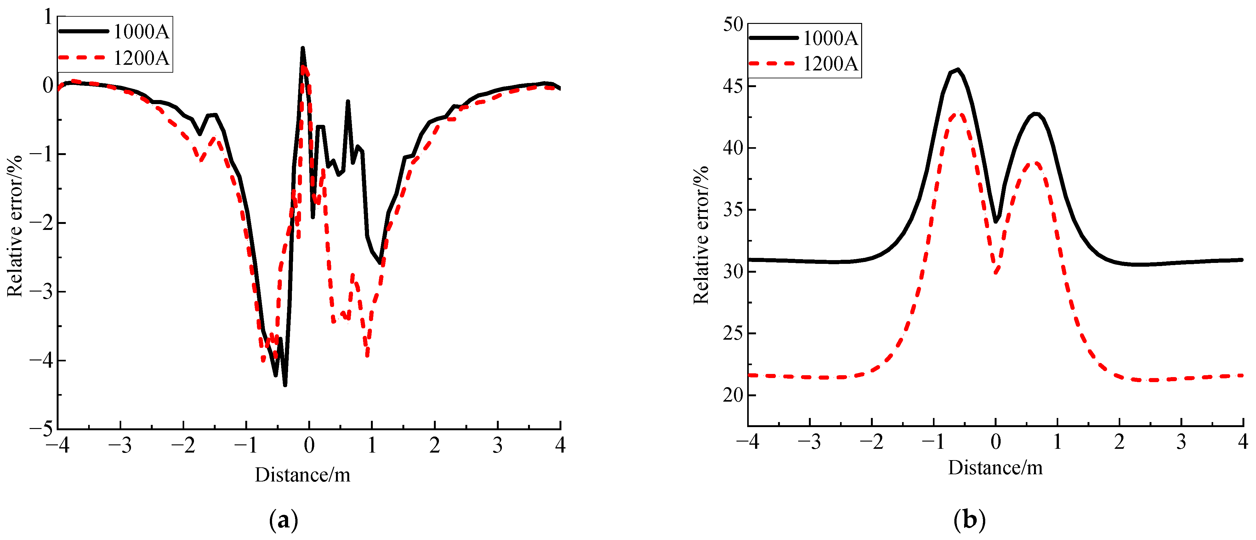
To further demonstrate the accuracy of the improved method, the result errors of both the improved method and the TEA method compared with the FEA method are shown in Figure 9a and Figure 9b, respectively. Figure 9a shows that the improved method results are basically lower than the simulation results, and the error is less than 5%, which can meet the requirements of engineering practice. The conductor temperature distribution curve obtained by the improved method is in good agreement with that obtained by the FEA method. Figure 9b shows that the TEA method results differ greatly from the simulation results, with the maximum error reaching 46%. Thus, the improved method can greatly improve the calculation accuracy of the conductor temperature of the cable joint, and realize an accurate thermal evaluation of the cable joint.

6. Conclusions

This paper proposed an improved method for cable joint thermal rating. In the improved method, the quasi-three-dimensional thermal model of the cable joint was developed and the conductor temperature distribution was obtained. The results of the improved method showed a good agreement with that of the FEA method, and the goodness of fit between the two method results achieved 0.97. Moreover, the error of the improved method with respect to the FEA method was less than 5%, while the maximum error of the TEA method reached 46%. The results demonstrate that the improved method is more suitable for accessing the thermal rating of the cable joint. The improved thermal rating method in this paper is easy to use and efficient for operating condition monitoring of cable joints in the field.

References

- Shabani, H.; Vahidi, B. A probabilistic approach for optimal power cable ampacity computation by considering uncertainty of parameters and economic constraints. Int. J. Electr. Power Energy Syst. 2019, 106, 432–443. [Google Scholar] [CrossRef]
- Xie, Y.; Liu, G.; Zhao, Y.; Li, L.; Ohki, Y. Rejuvenation of Retired Power Cables by Heat Treatment. IEEE Trans. Dielectr. Electr. Insul. 2019, 26, 668–670. [Google Scholar] [CrossRef]
- Liu, S.; Kopsidas, K. Risk-Based Underground Cable Circuit Ratings for Flexible Wind Power Integration. IEEE Trans. Power Deliv. 2021, 36, 145–155. [Google Scholar] [CrossRef]
- Vollaro, R.d.L.; Fontana, L.; Vallati, A. Thermal analysis of underground electrical power cables buried in non-homogeneous soils. Appl. Therm. Eng. 2011, 31, 772–778. [Google Scholar] [CrossRef]
- Wang, P.-Y.; Ma, H.; Liu, G.; Han, Z.-Z.; Guo, D.-M.; Xu, T.; Kang, L.-Y. Dynamic Thermal Analysis of High-Voltage Power Cable Insulation for Cable Dynamic Thermal Rating. IEEE Access 2019, 7, 56095–56106. [Google Scholar] [CrossRef]
- IEC 60287 Series; Electric Cables—Calculation of the Current Rating. International Electrotechnical Commission: Geneva, Switzerland, 2023.
- Nakamura, S.; Morooka, S.; Kawasaki, K. Conductor temperature monitoring system in underground power transmission XLPE cable joints. IEEE Trans. Power Deliv. 1992, 7, 1688–1697. [Google Scholar] [CrossRef]
- Gouda, O.; El, D.; Adel, Z. Electrothermal Analysis of Low- and Medium- voltage Cable Joints. Electr. Power Compon. Syst. 2016, 4, 110–121. [Google Scholar] [CrossRef]
- Liao, Y.; Bao, S.; Xie, Y.; Zhao, Y.; Wang, P.; Liu, G.; Hui, B.; Xu, Y. Breakdown failure analysis of 220 kV cable joint with large expanding rate under closing overvoltage. Eng. Fail. Anal. 2021, 120, 105086. [Google Scholar] [CrossRef]
- Bragatto, T.; Cerretti, A.; D’orazio, L.; Gatta, F.M.; Geri, A.; Maccioni, M. Thermal Effects of Ground Faults on MV Joints and Cables. Energies 2019, 12, 3496. [Google Scholar] [CrossRef]
- Yang, F.; Liu, K.; Cheng, P.; Wang, S.; Wang, X.; Gao, B.; Fang, Y.; Xia, R.; Ullah, I. The Coupling Fields Characteristics of Cable Joints and Application in the Evaluation of Crimping Process Defects. Energies 2016, 9, 932. [Google Scholar] [CrossRef]
- Gela, G.; Dai, J. Calculation of thermal fields of underground cables using the boundary element method. IEEE Trans. Power Deliv. 1988, 3, 1341–1347. [Google Scholar] [CrossRef]
- Wang, P.; Liu, G.; Ma, H.; Liu, Y.; Xu, T. Investigation of the Ampacity of a Prefabricated Straight-Through Joint of High Voltage Cable. Energies 2017, 10, 2050. [Google Scholar] [CrossRef]
- Quan, L.; Fu, C.; Si, W.; Yang, J. Numerical study of heat transfer in underground power cable system. In Proceedings of the 10th International Conference on Applied Energy (ICAE2018), Hong Kong, China, 22–25 August 2018; pp. 5317–5322. [Google Scholar]
- Pilgrim, J.A.; Swaffield, D.J.; Lewin, P.L.; Larsen, S.T.; Payne, D. Assessment of the Impact of Joint Bays on the Ampacity of High-Voltage Cable Circuits. IEEE Trans. Power Deliv. 2009, 24, 1029–1036. [Google Scholar] [CrossRef]
- Yang, F.; Cheng, P.; Luo, H.; Yang, Y.; Liu, H.; Kang, K. 3-D thermal analysis and contact resistance evaluation of power cable joint. Appl. Therm. Eng. 2016, 93, 1183–1192. [Google Scholar] [CrossRef]
- Ruan, J.-J.; Liu, C.; Huang, D.-C.; Zhan, Q.-H.; Tang, L.-Z. Hot spot temperature inversion for the single-core power cable joint. Appl. Therm. Eng. 2016, 104, 146–152. [Google Scholar] [CrossRef]
- Aziz, M.M.A.; Riege, H. A New Method for Cable Joints Thermal Analysis. IEEE Trans. Power Appar. Syst. 1980, PAS-99, 2386–2392. [Google Scholar] [CrossRef]
- Bragatto, T.; Cresta, M.; Gatta, F.; Geri, A.; Maccioni, M.; Paulucci, M. A 3-D nonlinear thermal circuit model of underground MV power cables and their joints. Electr. Power Syst. Res. 2019, 173, 112–121. [Google Scholar] [CrossRef]
- Bragatto, T.; Cresta, M.; Gatta, F.; Geri, A.; Maccioni, M.; Paulucci, M. Underground MV power cable joints: A nonlinear thermal circuit model and its experimental validation. Electr. Power Syst. Res. 2017, 149, 190–197. [Google Scholar] [CrossRef]
- Pilgrim, J.; Swaffleld, D.; Lewin, P.; Payne, D. An Investigation of Thermal Ratings for High Voltage Cable Joints through the use of 2D and 3D Finite Element Analysis. In Proceedings of the 2008 IEEE International Symposium on Electrical Insulation, Vancouver, BC, Canada, 9–12 June 2008; pp. 543–546. [Google Scholar]
- Bustamante, S.; Mínguez, R.; Arroyo, A.; Manana, M.; Laso, A.; Castro, P.; Martinez, R. Thermal behaviour of medium-voltage underground cables under high-load operating conditions. Appl. Therm. Eng. 2019, 156, 444–452. [Google Scholar] [CrossRef]
- Holyk, C.; Liess, H.-D.; Grondel, S.; Kanbach, H.; Loos, F. Simulation and measurement of the steady-state temperature in multi-core cables. Electr. Power Syst. Res. 2014, 116, 54–66. [Google Scholar] [CrossRef]
- Degefa, M.Z.; Lehtonen, M.; Millar, R.J. Comparison of Air-Gap Thermal Models for MV Power Cables Inside Unfilled Conduit. IEEE Trans. Power Deliv. 2012, 27, 1662–1669. [Google Scholar] [CrossRef]
- Anders, G.J. Rating of Electric Power Cables in Unfavorable Thermal Environment; Wiley: Hoboken, NJ, USA, 2005. [Google Scholar]
- Chippendale, R.D.; Pilgrim, J.A.; Goddard, K.F.; Cangy, P. Analytical Thermal Rating Method for Cables Installed in J-Tubes. IEEE Trans. Power Deliv. 2016, 32, 1721–1729. [Google Scholar] [CrossRef]
- Liu, G.; Xu, Z.; Ma, H.; Hao, Y.; Wang, P.; Wu, W.; Xie, Y.; Guo, D. An improved analytical thermal rating method for cables installed in short-conduits. Int. J. Electr. Power Energy Syst. 2020, 123, 106223. [Google Scholar] [CrossRef]
- Lemoine, C.; Besnier, P.; Drissi, M. Investigation of Reverberation Chamber Measurements Through High-Power Goodness-of-Fit Tests. IEEE Trans. Electromagn. Compat. 2007, 49, 745–755. [Google Scholar] [CrossRef]
Figure 1.
Quarter-element thermal model of cable joint.
Figure 2.
Cable joint 2D simulation model: 1—Block, 2—Copper shell, 3—Filling glue, 4—PVC belt, 5—Joint main insulation, 6—Copper screen tube, 7—Connection tube, 8—Air gap, 9—Shielding tube, 10—Conductor, 11—XLPE insulation, 12—Buffer layer, 13—Air gap, 14—Aluminum sheath, 15—Outer sheath.
Figure 3.
Schematic diagram of temperature sampling path.
Figure 4.
Temperature distribution results of the cable joint under different loads. (a) Conductor temperature, and (b) Surface temperature. Note: ①—the load is 1250 A, ②—the load is 1200 A, ③—the load is 1100 A, ④—the load is 1000 A, ⑤—the load is 900 A.
Figure 5.
Segment diagram of cable joint.
Figure 6.
The quasi-3D thermal model of the long end of the cable joint. Note: ΔTh1~ΔThj is the radial thermal resistance of shielding tube, ΔTm1~ΔTmk is the radial thermal resistance of cable joint main insulation, ΔTp1~ΔTpm is the radial thermal resistance of PVC belt, ΔTs1~ΔTsm is the radial thermal resistance of sealant, ΔTc1~ΔTcm is the radial thermal resistance of copper shell, ΔTi(j+1)~ΔTin is the radial thermal resistance of XLPE insulation, ΔTw(m+1)~ΔTwn is the radial thermal resistance of buffer layer, ΔTsh(m+1)~ΔTshn is the radial thermal resistance of aluminum sheath, ΔTo(m+1)~ΔTon is the radial thermal resistance of outer sheath, ΔTx1~ΔTxn is the axial unit thermal resistance of conductor, θ1′~θm′ is the surface temperature of cable joint, θ(m+1)′~θn′ is the surface temperature of cable, θ1~θm is the conductor temperature of cable joint, θ(m+1)~θn is the conductor temperature of cable, and ΔQr1~ΔQn is the conductor loss.
Figure 7.
Simplified quasi-3D thermal model of the long end of the cable.
Figure 8.
Comparison of theoretical and simulation results. (a) the load is 1000 A, and (b) the load is 1200 A.
Figure 9.
Error analysis for different methods. (a) error of the improved method, and (b) error of the TEA method.