
Short-Term Load Forecasting Based on Optimized Random Forest and Optimal Feature Selection


IT—Instituto de Telecomunicações, University of Beira Interior, 6201-001 Covilhã, Portugal
*
Author to whom correspondence should be addressed.
Energies 2024, 17(8), 1926; https://0-doi-org.brum.beds.ac.uk/10.3390/en17081926
Submission received: 6 March 2024
/
Revised: 10 April 2024
/
Accepted: 12 April 2024
/
Published: 18 April 2024
(This article belongs to the Topic Short-Term Load Forecasting)
Abstract
:Short-term load forecasting (STLF) plays a vital role in ensuring the safe, efficient, and economical operation of power systems. Accurate load forecasting provides numerous benefits for power suppliers, such as cost reduction, increased reliability, and informed decision-making. However, STLF is a complex task due to various factors, including non-linear trends, multiple seasonality, variable variance, and significant random interruptions in electricity demand time series. To address these challenges, advanced techniques and models are required. This study focuses on the development of an efficient short-term power load forecasting model using the random forest (RF) algorithm. RF combines regression trees through bagging and random subspace techniques to improve prediction accuracy and reduce model variability. The algorithm constructs a forest of trees using bootstrap samples and selects random feature subsets at each node to enhance diversity. Hyperparameters such as the number of trees, minimum sample leaf size, and maximum features for each split are tuned to optimize forecasting results. The proposed model was tested using historical hourly load data from four transformer substations supplying different campus areas of the University of Beira Interior, Portugal. The training data were from January 2018 to December 2021, while the data from 2022 were used for testing. The results demonstrate the effectiveness of the RF model in forecasting short-term hourly and one day ahead load and its potential to enhance decision-making processes in smart grid operations.
1. Introduction
Electrical load forecasting is a fundamental aspect for power suppliers, as it ensures the safe, effective, and economical operation of a power system. This forecasting practice is categorized into four types based on forecasting time: very short-term, short-term, medium-term, and long-term load forecasting [1]. Short-term load forecasting (STLF) is particularly important because it covers a forecast horizon of a few hours to a few days, allowing for the planning of generation resources, the optimization of power flow on the transmission grid, and the successful trading of power in the markets [2].
The complexity of STLF derives from several factors, including non-linear trends, multiple seasonality, variable variance, significant random interruptions, and variable daily profiles in electricity demand time series. Profiles have become more complex over the years. Together with the upcoming green revolution in power systems, they will certainly present added challenges [3], requiring advanced models to capture the hard non-linear characteristics and deliver accurate load predictions [4].
Accurate load forecasting offers numerous advantages for electric utilities, such as reduced operational and maintenance costs, increased reliability, and informed decisions for future development [5]. In addition, accurate load forecasting is essential in competitive power markets, where electricity prices are driven by demand, directly affecting the financial performance of market participants [6].
Improving the accuracy of short-term load forecasting is a challenging task but is of great value in ensuring safe and stable power system operation. Even a small increase in forecast accuracy can lead to substantial profits, making accurate, high-speed forecasting crucial for economic load dispatch in power systems [7]. Thus, the development of an efficient short-term load forecasting model is very important for smart grid operations and enhances decision-making processes [8,9]. This is particularly true for more disaggregated loads (as studied in this work), which usually constitute a more substantial challenge with higher forecasting errors [10].
1.1. Literature Review: Forecasting Models
A vast array of research exists on the prediction of time series data, encompassing various fields and presenting a multitude of proposed approaches. These methodologies strive to effectively capture the connections between future values of the predicted variable (output) and past data related to various influencing factors, which may include the predicted variable itself (input) [11].
In the past, conventional models such as autoregressive integrated moving average (ARIMA) or exponential smoothing were widely regarded as effective techniques for capturing the internal dependencies within the forecast variable. These models were part of the hard computing paradigm [12], and, to mitigate some of their shortcomings, they have been effectively integrated into assembled STLF models [13]. The adoption of artificial intelligence (AI) techniques has become increasingly prevalent in various fields, including in forecasting models [14], a trend that is also driven by data proliferation, including in this field, where increasingly disaggregated levels of load time series and related variables are now available for customers, researchers, etc. The characteristics of these time series determine different input selection and processing approaches, which are both key for the training and fine-tuning of these models [15].
In the context of the power system, AI can help operators maximize profit by forecasting electric load and electricity prices. Conventional machine learning models such as support vector machines [16], regression models [17], random forest (RF) [1], decision trees [18], extreme gradient boosting (XGBoost) [19], and AI models such as artificial neural networks (ANNs) [20] are commonly used to solve electrical engineering problems, in particular electricity load forecasting. Different types of artificial neural networks have been explored, including feedforward and recurrent neural networks, e.g., Elman networks, Jordan networks, long-short term memory (LSTM), and gated recurrent unit (GRU) neural networks] and convolutional neural networks [21,22]. In addition, many authors prefer to use hybrid models, combining two or more models [23,24,25,26].
Given the complexities of electricity demand time series, machine learning (ML) methods are the preferred class of electricity demand forecasting method [27]. Random forest (RF)—an ensemble learning method for both regression and classification problems—was presented by [28] in regression problems and has been one of the most popular machine learning (ML) models. The RF algorithm has been applied efficiently and extensively in several works that involve long-, medium-, short-, and ultra-short-term forecasting. Some recent approaches, namely electricity load forecasting, have been applied to the electricity sector. In [29], a hybrid RF–MGF–RSM model is proposed for short-term forecasting, combining random forest with the averaging function. In [30], medium-term models for isolated power systems are applied, exploring machine learning methods such as random forest and XGBoost. In contrast, ref. [31] proposes a hybrid feature selection algorithm for short-term forecasting, integrating genetic algorithms and random forest. Meanwhile, ref. [32] highlights an ultra-short-term forecasting model that combines LSTM and random forest. The authors in [33] have developed a long-term forecasting system based on knowledge and data, using machine learning regression methods and inference based on fuzzy logic. These recent works highlight a variety of approaches and forecasting horizons for electricity load, from the short to the long term, exploring different machine learning techniques and models.
1.2. Contributions
In a framework where consumers are expected to manage their electrical loads more actively, it is important to tackle the issue of STLF at a more decentralized level, including high-consumption public buildings. These entities can, thereby, best understand their consumption patterns, adjust their activities, consider different dynamic pricing options, and define a self-consumption plan with the possibility of storage [34]. This more proactive role requires accurate STLF as a crucial task for a better decision-making process. Therefore, in this work, we will delve into the main issues surrounding this goal, specifically by acknowledging that a one-size-fits-all approach is not the correct path and that we should pursue a more tailored input data selection coupled with forecasting model fine-tuning.
The main contributions of this paper can be summarized as follows: (i) the selection of features combined with exogenous variables—such as calendar (hour and weekday) and temperature—allowed us to find an optimal and customized combination for each case study. This analysis proved that, regardless of the forecasting model used, it is essential to explore several types of input variables to find the most significant one; (ii) the study of the correlation between weekdays showed that, although highly correlated, replacing weekdays will not necessarily improve result accuracy; (iii) hyperparameter tuning showed that there is no single optimal parameterization for all consumption profiles, i.e., each case study obtained the best results from different parameter settings. This proves that hyperparameter tuning is fundamental to improve results; (iv) contrary to expectation, training with rolling forecast showed benefits in only one case study; in the others, introducing recent information and removing older information did not improve the results. Thus, this analysis proves that the use of rolling forecast improves forecast accuracy depending on the consumption profile; (v) since there is no consensus in the literature on the use of an optimal forecasting model for STLF, this paper used the RF model, which in most cases resulted in the more accurate forecasts when compared to baseline models.
1.3. Paper Structure
In this paper, Section 2 presents the proposed forecast model and the input data selection as well as the exogenous variables used for training. Section 3 presents a brief statistical analysis of the data and provides the results of various experiments, including similar weekday, tuning hyperparameter, rolling forecast, and a comparative baseline model. Lastly, Section 4 presents the main conclusions.
2. Proposed Forecast Model
2.1. Input Data Selection
Electricity load time series express random fluctuations, trends, and seasonality on an annual, weekly, and daily basis. The daily load profiles are dependent on the day of the week and the hour of the day and vary throughout the year. These components will depend on system size and structure, as well as weather conditions. In this study, the STLF model produced hourly forecasts one day ahead (hour of day ). For this purpose, the predictors used as input for the forecast model should be the most relevant variables, selected from recent history. Furthermore, data processing is fundamental to reducing forecast errors.
To obtain the most accurate forecast possible, the time series input patterns should be the most representative of the time series. Thoughtful data selection allows for maximizing the accuracy and reliability of the analysis or model. Furthermore, by selecting relevant data, it is possible to reduce noise and bias in the results, optimize the use of computational resources, and facilitate scalability and generalization of the model. This leads to deeper insights, more reliable decisions, and a better understanding of the behavior of the electrical system over time. Table 1 shows different input patterns with different combinations of relevant lags. The settings for some of these input patterns were inspired by [35].
Depending on the input pattern, you can introduce different input information into the model. Unlike , which only offers insights into daily seasonality, pattern contains comprehensive details about the weekly sequence leading up to the forecasted day . Notably, captures both daily and weekly seasonality. Patterns and consider the same hour that will be forecasted for the next day , but considering one and three the earlier weeks, respectively, expressing only weekly seasonality.
Pattern considers only the hour of the seven last same weekdays as the forecasted day . For example, if the weekday to be forecasted is a Sunday, the sequence will be the hour of the seven preceding Sundays. Pattern selects some of the lags generally considered the most relevant and, in addition, the previous and subsequent hours. For example, for lag 24, it also considered hours 23 and 25. This pattern reduces the number of relevant lags while prioritizing recent information from up to a week ago.
Cross-patterns and are a combination of patterns and , respectively, that consider daily as well as weekly seasonality. In [35], the authors demonstrated that combining daily and weekly patterns in STLF produces more favorable results than using individual daily or weekly patterns for forecasting.
Figure 1 shows the sequence of input patterns , , , , and ; Figure 2 shows the sequence of input cross-patterns and and Figure 3 show the representation of these input patterns.
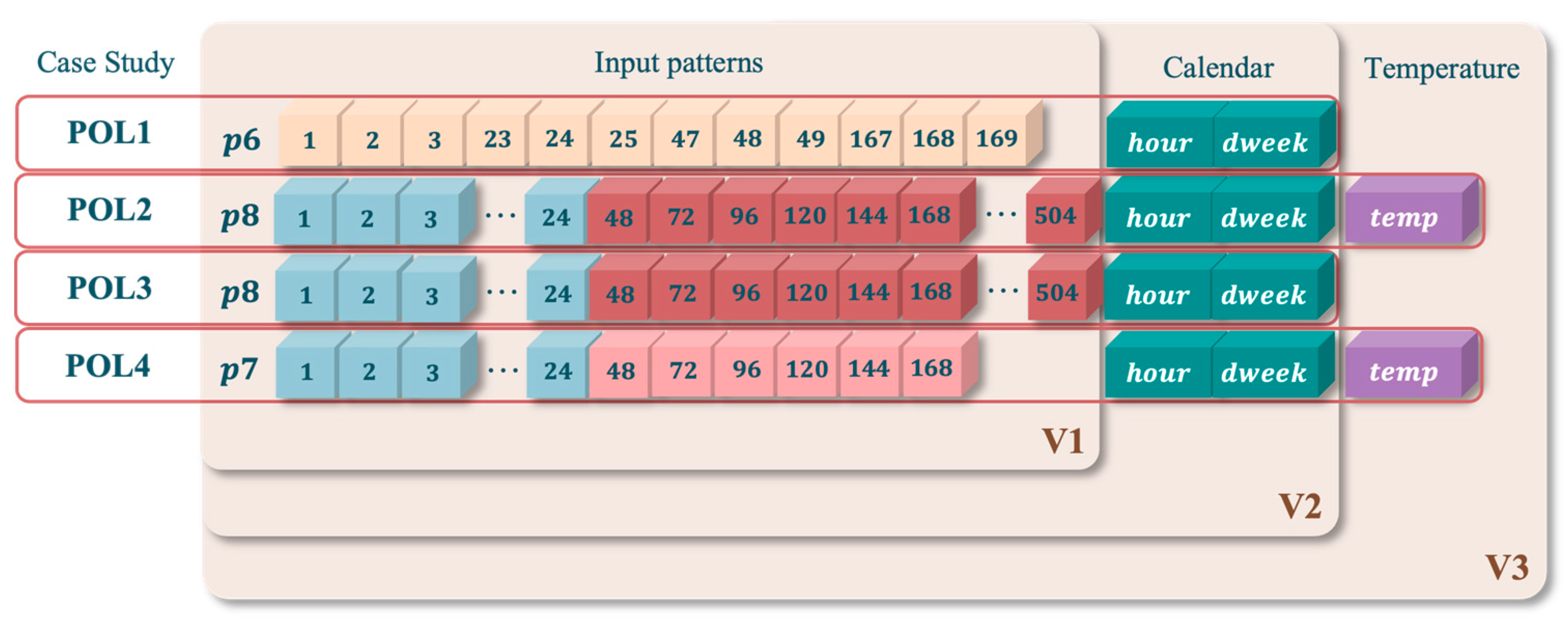
To explore multiple prediction performances, we used three different variants of input data for model training. Variant 1 only included load information, namely an input pattern () and the target (24 h ahead). Variant 2 also included calendar variables, namely hour of the day and day of the week , both categorical variables. Variant 3 added ambient temperature in Celsius () as an exogenous variable. Figure 4 represents these variants schematically.
2.2. Forecasting Model: Random Forest (RF)
Random forest (RF) is an ensemble algorithm based on a decision tree model (CART—classification and regression trees) [36]. The main idea of the RF model is to create a random combination of regression trees, using techniques such as bagging [37] and random subspace [38]. In bagging, each tree in the forest is built from a bootstrap sample (sampling with replacement) of the original dataset. The random subspace technique, in addition to bagging, randomly selects a certain number of features to be sampled, increasing the diversity among trees, since it creates random subsets of the complete predictor space (more specifically, a random predictor subset is selected at each tree node). When combined, these techniques improve prediction accuracy and reduce model variability.
The RF algorithm uses a bootstrap sample () with the same size as the training data for each of trees (). For each sample, a tree is constructed by recursively partitioning the input space at each node until a minimum sample leaf size is reached. At each node, splits are based on randomly chosen features () from among the total number of features (). The best split is chosen by maximizing the reduction of the mean square error (MSE) among all split candidates and cut points. After all trees are constructed in this way, the RF forecast can be calculated by (1) [39]:
where is the input pattern.
Some hyperparameters can be settled to improve the forecasting results, such as the number of trees (), the minimum sample leaf size () and the number of maximum features to select at random for each split (). For regression problems, the literature recommends that the number of maximum features should be the total number of features () divided by 3, because as decreases, the correlation between trees decreases and, with this, the variation of the mean also decreases.
The best values for the hyperparameters will always depend on each problem. In this case study, these parameters were initially set as , and . Pseudocode of the random forest algorithm is described in Algorithm 1.
| Algorithm 1: Pseudocode of the Random Forest algorithm. |
| Input: Training data. . . . Procedure: Select a bootstrap sample randomly of the same size as the training data. is reached: Step 1: Select n features randomly from all features. Step 2: From these randomly selected n features, choose the best feature that splits the data to compose the current node. Step 3: Split the node into two other nodes. Output: . Calculate the forecast of point : |
3. Simulation Study
3.1. Statistical Analysis of Data
Historical hourly load data (active power demand [kW]) from 4 transformer substations that supply the distribution grid of four campuses of the University of Beira Interior-UBI, located in Covilhã (Portugal), were used to test the proposed forecast model. Four case studies were chosen: the Sciences and Humanities campus (represented in this paper by POL1), the Mathematics and Informatics campus (POL2), the Engineering campus (POL3), and the Health Sciences campus (POL4). The data comprised the period from January 2018 to December 2022. Figure 5 represents the average hourly consumption per month and per year for each campus. The data from 2018 to 2021 were used for training, and 2022 was used for testing.
Figure 6 presents the descriptive statistics of the load data from the training and testing periods. Null power data were taken from the database, but POL3 still showed very low minimum load values of 1kW. The mean values were similar for both periods, except for POL3, which had a lower mean value in the test period. Clearly, POL4 has the highest consumption among all campuses. The standard deviation (SD) was higher in the testing period only for POL4; the same was true for the maximum values. Statistically, the test period resembled the training period, showing that the data were consistent to test the proposed forecast model.
3.2. Results for All Configurations of Input Patterns and Training Modes
The forecast error was calculated using the mean absolute percentage error (MAPE) and root mean square error (RMSE). These error metrics can be calculated by (2) and (3), respectively. Table 2 and Table 3 show the MAPE and RMSE, respectively, for input patterns and different training variants.
Variant 1, which only used load data, achieved the worst result for each input pattern tested in all case studies. The highest errors for Variant 1 were observed with patterns and and the lowest errors were observed with pattern . Variant 2, which adds calendar information (hour and weekday) reduced the error in all cases. Variant 2 presented the lowest errors when combined with patterns for POL1 and for POL3. In some cases, Variant 3, which adds temperature information, reduced the error. For this variant, the best options were combining patterns for POL2 and for POL4. The RMSE values for POL4 were greater than for the other case studies due to relatively higher consumption compared to the other campuses, as shown in Figure 6.
where is the real value; is the forecast value; and is total number of observations.
Based on the results, a different combination is recommended for each case study. The best combination for POL1 and POL3 is Variant 2 with patterns and , respectively, while for POL2 and POL4, the best combination is Variant 3 with patterns and , respectively. For POL1 and POL3, where temperature data are not required, the load profiles are less sensitive to temperature variations, either due to specific characteristics of the data or the forecasting method that effectively captured variation in electricity demand without the need to include temperature data. In fact, the correlation values between temperature and electricity demand were relatively low, with values of −0.1 for POL1 and −0.2 for POL3. On the other hand, despite a correlation of −0.2, POL2 showed greater sensitivity to climate variations, which is why the forecasting model favored a combination that includes the temperature. In the case of POL4, the best combination confirmed the expectations given by the correlation between temperature and electricity demand, with a significant value of 0.6, which is why the temperature data were also included. This suggests that clear variations in ambient temperature, such as a hotter summer or a colder winter, directly influence the amount of electricity consumed. Figure 7 illustrates the best combination among all results for each case study. These combinations were used in the next subsections.
3.3. Results for Best Configuration: Similar Weekday
In addition to seasonality, energy consumption among university campuses is similar across weekdays. Certain days are highly correlated, such as Saturday and Sunday (weekend), when academic activity is reduced and consequently energy consumption is lower.
To improve the forecast results, an analysis of the correlation between the days of the week was performed using Pearson’s coefficient (). Figure 8 shows the correlation matrix for each case study. There is clearly a high correlation between certain days of the week. Consequently, the code for the calendar variable —initially, 1 for Sunday, 2 for Monday and so on—was changed to 1 for Saturday and Sunday; 2 for Monday and Tuesday; and 3 for Wednesday, Thursday, and Friday.
Contrary to expectation, the use of similar weekdays did not prove relevant, as prediction error did not decrease when compared to the initial result. Table 4 shows the MAPE and RMSE values for both cases.
3.4. Tuning the Hyperparameters
Hyperparameter tuning is a critical step in the development of machine learning models. The selection of appropriate hyperparameters can profoundly impact model performance, influencing its ability to generalize well to unseen data and achieve optimal predictive accuracy. Failure to select hyperparameters accurately or adequately can lead to sub-optimal model performance, even with state-of-the-art algorithms. Therefore, understanding and effectively addressing the hyperparameter tuning process are imperative to ensuring model effectiveness and reliability. The authors in [40] addresses challenges such as overfitting and parameter selection inherent to standard methods based on artificial neural networks (ANNs).
To improve the accuracy of the forecast, the parameters , , and were adjusted. Details of each of these parameters are presented below, highlighting the advantages and disadvantages of setting them:
- The number of trees (): This parameter defines the number of trees in the forest. It is an essential parameter that significantly influences the model’s performance. Increasing the number of trees offers several advantages, including reducing the variability of the model, leading to more consistent prediction errors and improving prediction accuracy. This increased robustness allows the model to better capture complex patterns in the data and generalize well to unseen instances, improving its overall forecasting capabilities. However, setting too low can result in underfitting, where the model fails to adequately capture essential patterns in the data, leading to sub-optimal prediction performance. On the other hand, setting too high can lead to longer training times without significant improvements in prediction accuracy, potentially wasting computational resources. It is therefore crucial to find the optimal value for , striking a balance between model complexity, computational efficiency and prediction performance.
- The minimum sample leaf size (): This parameter controls the minimum size of the leaves in the tree. It is a fundamental parameter in the construction of decision trees. Adjusting the minimum size of the leaves in the tree appropriately is essential in reducing uncertainty in decision-making. A significant advantage of setting this parameter is the ability to avoid forming excessively deep trees, which, although they may have small biases, also tend to have high variability. However, this setting can result in models with a larger bias and a loss of fine detail in the data. It is therefore essential to find a balance when adjusting this parameter, in order to mitigate uncertainty without compromising the model’s ability to capture the complexity of the data and avoid overfitting.
- The maximum number of features selected randomly for each split (): This parameter is crucial in random forest algorithms. It determines the maximum number of features to be considered when splitting a node during the construction of each tree in the forest. Adjusting this parameter has significant implications for the performance and robustness of the model. One of the main advantages of adjusting this parameter is the introduction of randomness in the process of building the trees. Limiting the number of features considered at each split reduces the correlation between the trees, making the model more robust and less prone to overfitting the training data. This is especially important to ensure that the model generalizes well to new data. Furthermore, adjusting this parameter allows for a customized adjustment of the model according to the specific characteristics of the dataset and the demands of the problem at hand. This provides flexibility in model tuning, allowing for a more precise adaptation to the problem’s needs. However, an improper choice of the value of n can lead to bias in the model. If n is too small, underfitting may occur, as the model may not be able to capture the complexity of the data. On the other hand, if n is too large, the model may become excessively complex, leading to overfitting. Therefore, it is essential to adjust this parameter carefully, seeking a balance between reducing overfitting and maintaining the model’s bias. Experimentation and careful adjustment are necessary to find the ideal value of n that optimizes the model’s performance and ensures good generalization to new data.
This subsection aims to provide transparency about the methodology used to adjust hyperparameters in this study. The exhaustive search method was applied to check all possible values of each hyperparameter within a given range.
Two different methods were used to optimize these hyperparameters. In one case, each hyperparameter was optimized individually, keeping the other hyperparameters constant, namely number of trees () = 300; minimum leaf size () = 1; and number of features to sample () = , where is the total number of features. In the second case, the hyperparameters were optimized simultaneously.
3.4.1. Tuning the Hyperparameters: Individually
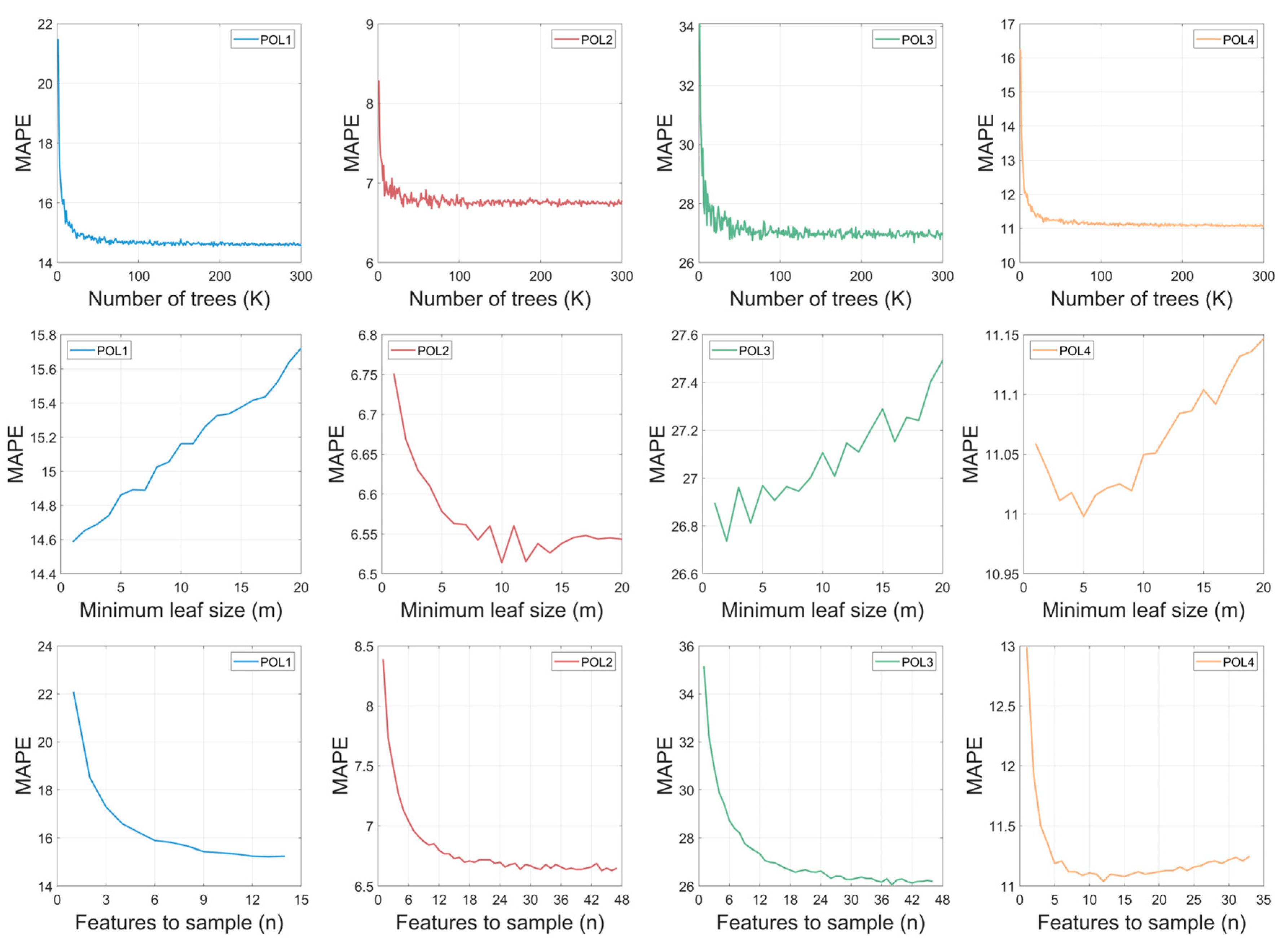
The range for the number of trees () was 1 to 300, and for minimum leaf size (), it was 1 to 20, for all case studies. The number of features to sample () was 1 to , where these values differed among case studies: 14 for POL1; 47 for POL2; 46 for POL3; and 33 for POL4. Figure 9 shows the impact of hyperparameters on the forecasting error (MAPE) for each case study. Regarding the number of maximum features to select at random for each split (), the optimal value was different for each case study: 13 for POL1; 46 for POL2; 38 for POL3; and 12 for POL4. For minimum leaf size (), the optimal value also differed among case studies: 1 for POL1; 10 for POL2; 2 for POL3; and 5 for POL4. Except for POL2, small values of were preferred.
MAPE remained constant with an increasing number of trees. To confirm this, the MAPE’s standard deviation (SD) was calculated considering a K between 100 and 300. The SD of the MAPE was low: 0.04 for POL1; 0.09 for POL3; and 0.02 for POL2 and POL4. In contrast, for the interval below 99 trees, the SD was higher: 0.88, 0.20, 0.95, and 0.64 for POL1 to POL4, respectively. Therefore, in the simultaneous optimization of the hyperparameters, the number of trees was kept fixed at = 300.
Table 5 shows the MAPE values for the best configuration for each individually tuned hyperparameter. POL1 showed the best configuration when only was optimized; however; the MAPE was the same as that obtained with the initial configuration (. POL2 and POL4, initially with , obtained the lowest MAPE when the value of was optimized, reducing the MAPE by 2% and 0.7%, respectively. POL3 showed the best result when optimizing the value of separately, obtaining the most significant reduction in MAPE (3.1%) compared with a MAPE of 26.89 obtained with the initial . Table 6 shows the MAPE values for the combinations of best hyperparameter values tuned individually and for the same tuned values of and n with . The MAPE value slightly decreased for POL1 and POL3 and remained the same for POL2 and POL4.
3.4.2. Tuning the Hyperparameters: Simultaneously
In this subsection, the number of trees was kept constant at and the MAPE was calculated for all possible combinations of and values within the range defined previously. Figure 10 shows, in 3 dimensions, the resulting MAPE for all combinations in each case study. Table 7 shows the MAPE and RMSE values for the initial and best configurations. Tuning the hyperparameters in a combined way reduced the MAPE by 3.8% for POL3 (the most significant reduction), by 3.3% for POL2, 2.6% for POL1 and 1.1% for POL4. The RMSE also decreased with tuned hyperparameters, except for POL1.
The bars shown in Figure 11 represent, for each case study, the absolute percentage difference in the mean hourly between the forecast and real values for the testing period. The percentage difference is calculated by the absolute value of 1 minus the ratio between the hourly average of the forecasted value and the real value. The colored areas behind the bars show the mean percentage difference for all the hours. Overall, POL4 had the lowest average percentage error of just 1.8%, representing an absolute error of 3.28 kW. Although POL1 had the highest average percentage error, of 2.6%, in absolute terms, it presented an error of 1.27kW, behind POL2 with 1.61kW and ahead of POL3, which had the smallest absolute average error of just 1.19kW.
3.5. Results of Training Using Monthly Rolling
A rolling forecast was used in this subsection. A rolling forecast predicts the load over a continuous period, based on historical data. Unlike static training and testing periods that forecast the load for a fixed time frame, e.g., January to December, a rolling forecast is regularly updated throughout the year to reflect any changes. In other words, the forecast is made for a certain month, and this is added to the training period as new information and is dropped one month after the training period.
Table 8 shows the MAPE and RMSE values for each month of 2022 trained using rolling forecasting. The mean value of all these months was compared with the forecast error without rolling training, using a fixed period for training, named Annual. Except for POL2, predictions were more accurate without rolling training.
POL1 presented MAPE values that were on average 19.2% higher than the annual MAPE value. The highest MAPE value was in April, a 105.9% increase relative to the annual; while the lowest MAPE was in September, 19.8% below the annual MAPE. For POL2, the rolling approach training reduced the mean MAPE values by 4.1% and mean RMSE value by 5.1%, compared to the annual values. Only three months had MAPE and RMSE values higher than the annual values. POL3 had a 280.1% increase in MAPE compared to the annual value in April, and a 42.2% reduction in October. Like POL1 and POL2, April was the worst month for predictions. This can be explained by April’s many holidays and reduced activity, unlike POL4. Between May and September, POL4 had MAPE values well above the mean. However, the training with rolling increased the mean MAPE values by 16% and mean RMSE value by just 1.7%. February was the only month that presented MAPE and RMSE values lower than the annual value for all case studies. Figure 12 shows the real load data and the forecasted value through this period, for all case studies.
3.6. Baseline Models Comparison
As a benchmark, five other well-known methods were used to predict the load 24 h ahead: the persistence method [41]; autoregressive moving average (ARMA) and autoregressive integrated moving average (ARIMA) [42]; artificial neural networks (ANNs) [43]; and extreme gradient boosting (XGBoost) [44]. Table 9 presents the main parameter setting for these baseline models, which were thoughtfully chosen to ensure their efficiency, as well as other main aspects of model implementation. All these models were tested using the same available training and testing data as the RF model.
The forecast results obtained by the RF model proposed in this paper were compared with those obtained by these comparison models, as shown in Table 10. The MAPE and RMSE values clearly show the benefits of the proposed forecasting model. For the testing dataset, the RF model was able to outperform most baseline models for all case studies. Figure 13 shows the percentage difference between the MAPE and RMSE values of each model tested compared to the proposed RF model.
The worst performance was given by the ARMA model for POL1 with a MAPE value of 70.03, representing a degradation of 394.6% relative to the proposed RF model. Considering the RMSE value, the worst performance was given by the ARIMA model, also for POL1. POL1 had the worst results for almost all the tested models compared to the other case studies. POL2 performed best with training using the ANN model, which reduced the MAPE value by 7.3% and the RMSE value by 4.4%. POL3 and POL4 had RMSE values using the XGBoost model that were very close to the RF model, with less than 1% degradation.
4. Conclusions
Power systems are undergoing an unprecedented transformation towards an environment where the consumer is empowered with a more proactive role, both by actively managing their electrical load and engaging in self-consumption. In other words, the advent of data-driven solutions for consumers, the significant cost reduction of photovoltaic technology, and the forthcoming maturation of modular energy storage solutions are evolving from the old paradigm of an “inelastic consumer” to a “flexible prosumer”, who is more prone to actively match their electrical load with off-peak pricing tariffs and/or to match their power production. Public buildings/services with significant loads (like hospitals, universities, and city halls, among others) will certainly be at the forefront of this transformation.
Reliable forecasting models constitute a key component of this proactive approach towards load management, guiding the decision-making process of consumers regarding their volatile electrical load. Short-term load forecasting represents the most important horizon in the exploration of this new paradigm and has therefore been the focus of researchers. Despite the countless approaches in the literature to individual and simultaneous load forecasting models, there is no hard consensus regarding these regression-type modelling problems. The limitations of every single approach demand comparing popular methods but also tailoring each model to the individual characteristics of the studied problem. Both data selection/processing sensitivity and fine-tuning model hyperparameters are a crucial part of any proposed STLF work.
In the present study, the electrical load from four university campuses (with different profiles and seasonality levels) were used to test the validity of a tailored forecasting approach. We began with the often-disregarded task of input selection and feature selection. Eight different input load patterns (sequences of relevant lags) were chosen for testing, each exploring different philosophies in terms of the targeted seasonalities; i.e., some explore only daily or weekly insights, while others target both. Thus, some patterns favored the autocorrelation function and continuity between the relevant lags, while others favored the lags with spikes in the partial autocorrelation function. This in turn leads to different input sizes. Then, recognizing the well-documented importance of exogenous variables, particularly calendar type variables, three different input variants were assembled for each of the eight input patterns, resulting in a total of 24 different input data selections for each of the four case studies.
With the input data prepared and having defined an initial forecasting model based on a RF model, we then trained the models with four years of data and determined which input data selection ensured the best forecasting accuracy in an entire year for each STLF case study. As expected, the results revealed an overall preference for the input data selection that targeted a mixture of daily and weekly relevant lags, but with a preference for sequences where only certain correlation spikes were present (p8, p7 and p6). Additionally, Variant 2—which includes weekday and hour as exogenous variables—ensured the lowest errors for POL1 and POL3. In contrast, Variant 3 revealed a greater forecasting accuracy for POL2 and POL4, underlining the benefits of considering temperature alongside the previous two calendar exogenous variables.
The results reveal significant changes in the MAPE and RMSE values according to input data selection, thus confirming the consensus regarding the use of typical exogenous variables for the considered STLF case studies. Nevertheless, the inferences from correlation analyses need to be confirmed in terms of the forecasting model, since the tested similar weekdays approach (reducing the input range of the weekday variable) did not improve forecasting accuracy. Testing all individual input data selections allowed us to pinpoint which input data selection to target in the subsequent hyperparameter optimization of the forecasting model for each STLF case study. This process was divided into two stages. First, the influence of hyperparameters was studied individually, highlighting some clear trends in the most influential hyperparameters and their range. In particular, we observed that, after a sharp decline, the forecasting error remained (almost) constant with an increasing number of trees; except for POL2, a smaller minimum leaf size was generally preferred; and regarding the features to sample, there were benefits of using larger values, with exponential reductions in forecasting error. Second, with these inferences, we proceeded to simultaneously optimize the hyperparameters, with the number of trees fixed at its upper bound. This revealed non-neglectable forecasting improvements for all case studies, in comparison with the results obtained by the initial RF model for the best input data selection configuration. A monthly rolling training and testing approach was also tested to check if it produced better results than the static approach. However, except for POL2, this did not improve the overall annual MAPE and RMSE error value. Nevertheless, it allowed us to identify the most problematic testing months and to conjecture about the reasons behind some of these larger errors, namely a connection with holidays and intra-year seasonalities, which, interestingly, were not present in every university campus load profile.
To complete the work, a baseline comparison with other well-established models was performed to underscore the relative superiority of the proposed approach based on an optimized RF model with tailored input data. Considering all the case studies, XGBoost was the closest baseline model, with an average MAPE and RMSE percentual difference of 5.2% and 1.6%, respectively. The ANN was the only model able to outscore the proposed RF model for POL2, although its MAPE and RMSE were worse by 12.0% and 11.2%, respectively, in terms of average percentage.
Finally, these results have validated the proposed forecasting approach by comprehensively studying the influence of the selected exogenous variables, correlation spikes and the model hyperparameters on the fine-tuning of the RF based load forecasting. We thus fulfilled our goals of taking advantage of the historical data and delivering a relatively simple-to-implement, and accurate, forecasting model that can be used by institutions like universities, in order to better predict their loads, adapt their patterns, and adjust their energy contracts, and in the near future, position themselves as active prosumers to take advantage full advantage of the green transition.
5. Future Works
Future research could explore the application of the proposed method for different types of applications, such as industrial or residential load forecasting. The extension of the model to encompass a broader range of load profiles and consumption patterns would provide valuable insights into the adaptability and robustness of the forecasting approach. Additionally, investigating the integration of real-time data sources, such as weather forecasts and market pricing, could enhance the model’s accuracy and applicability in dynamic energy environments. Furthermore, the exploration of hybrid forecasting models, combining the random forest algorithm with other advanced techniques such as artificial neural networks or XGBoost, could lead to improved forecasting performance across diverse energy consumption scenarios. Lastly, the potential integration of the proposed forecasting model into smart grid systems and demand response programs warrants further investigation to assess its effectiveness in supporting grid stability and facilitating efficient energy management.
Author Contributions
Conceptualization, B.M.; methodology, B.M., P.B. and S.M.; validation, B.M., P.B. and M.d.R.C.; formal analysis, B.M., P.B., J.P., M.d.R.C. and S.M.; investigation, B.M., P.B., J.P., M.d.R.C. and S.M.; resources, M.d.R.C. and S.M.; writing—original draft preparation, B.M.; writing—review and editing, B.M., P.B. and M.d.R.C.; visualization, B.M., P.B., J.P., M.d.R.C. and S.M.; supervision, M.d.R.C. and S.M. All authors have read and agreed to the published version of the manuscript.
Funding
This research received no external funding.
Data Availability Statement
The original contributions presented in the study are included in the article, further inquiries can be directed to the corresponding author.
Acknowledgments
Bianca Magalhães gives his special thanks to the Fundação para a Ciência e a Tecnologia (FCT), Portugal, for the Ph.D. Grant (2023.02678.BDANA).
Conflicts of Interest
The authors declare no conflicts of interest.
References
- Veeramsetty, V.; Reddy, K.R.; Santhosh, M.; Mohnot, A.; Singal, G. Short-Term Electric Power Load Forecasting Using Random Forest and Gated Recurrent Unit. Electr. Eng. 2022, 104, 307–329. [Google Scholar] [CrossRef]
- Holderbaum, W.; Alasali, F.; Sinha, A. Short Term Load Forecasting (STLF). Lect. Notes Energy 2023, 85, 13–56. [Google Scholar] [CrossRef]
- Pinheiro, M.G.; Madeira, S.C.; Francisco, A.P. Short-Term Electricity Load Forecasting—A Systematic Approach from System Level to Secondary Substations. Appl. Energy 2023, 332, 120493. [Google Scholar] [CrossRef]
- Akhtar, S.; Shahzad, S.; Zaheer, A.; Ullah, H.S.; Kilic, H.; Gono, R.; Jasí Nski, M.; Leonowicz, Z. Short-Term Load Forecasting Models: A Review of Challenges, Progress, and the Road Ahead. Energies 2023, 16, 4060. [Google Scholar] [CrossRef]
- Yang, D.; Guo, J.; Li, Y.; Sun, S.; Wang, S. Short-Term Load Forecasting with an Improved Dynamic Decomposition-Reconstruction-Ensemble Approach. Energy 2023, 263, 125609. [Google Scholar] [CrossRef]
- Leal, P.; Castro, R.; Lopes, F. Influence of Increasing Renewable Power Penetration on the Long-Term Iberian Electricity Market Prices. Energies 2023, 16, 1054. [Google Scholar] [CrossRef]
- Xia, Y.; Wang, J.; Wei, D.; Zhang, Z. Combined Framework Based on Data Preprocessing and Multi-Objective Optimizer for Electricity Load Forecasting. Eng. Appl. Artif. Intell. 2023, 119, 105776. [Google Scholar] [CrossRef]
- Dewangan, F.; Abdelaziz, A.Y.; Biswal, M. Load Forecasting Models in Smart Grid Using Smart Meter Information: A Review. Energies 2023, 16, 1404. [Google Scholar] [CrossRef]
- Alquthami, T.; Zulfiqar, M.; Kamran, M.; Milyani, A.H.; Rasheed, M.B. A Performance Comparison of Machine Learning Algorithms for Load Forecasting in Smart Grid. IEEE Access 2022, 10, 48419–48433. [Google Scholar] [CrossRef]
- Groß, A.; Lenders, A.; Schwenker, F.; Braun, D.A.; Fischer, D. Comparison of Short-Term Electrical Load Forecasting Methods for Different Building Types. Energy Inform. 2021, 4, 13. [Google Scholar] [CrossRef]
- Wang, F.; Li, K.; Zhou, L.; Ren, H.; Contreras, J.; Shafie-khah, M.; Catalão, J.P.S. Daily Pattern Prediction Based Classification Modeling Approach for Day-Ahead Electricity Price Forecasting. Int. J. Electr. Power Energy Syst. 2019, 105, 529–540. [Google Scholar] [CrossRef]
- Pourdaryaei, A.; Mohammadi, M.; Karimi, M.; Mokhlis, H.; Illias, H.A.; Kaboli, S.H.A.; Ahmad, S. Recent Development in Electricity Price Forecasting Based on Computational Intelligence Techniques in Deregulated Power Market. Energies 2021, 14, 6104. [Google Scholar] [CrossRef]
- Bento, P.M.R.; Pombo, J.A.N.; Calado, M.R.A.; Mariano, S.J.P.S.; Rodrigues, F.; Calado, J.M.F. Stacking Ensemble Methodology Using Deep Learning and ARIMA Models for Short-Term Load Forecasting. Energies 2021, 14, 7378. [Google Scholar] [CrossRef]
- Shi, J.; Li, C.; Yan, X. Artificial Intelligence for Load Forecasting: A Stacking Learning Approach Based on Ensemble Diversity Regularization. Energy 2023, 262, 125295. [Google Scholar] [CrossRef]
- Du, J.; Cao, H.; Li, Y.; Yang, Z.; Eslamimanesh, A.; Fakhroleslam, M.; Mansouri, S.S.; Shen, W. Development of hybrid surrogate model structures for design and optimization of CO2 capture processes: Part I. Vacuum pressure swing adsorption in a confined space. Chem. Eng. Sci. 2024, 283, 119379. [Google Scholar] [CrossRef]
- Rao, C.; Zhang, Y.; Wen, J.; Xiao, X.; Goh, M. Energy Demand Forecasting in China: A Support Vector Regression-Compositional Data Second Exponential Smoothing Model. Energy 2023, 263, 125955. [Google Scholar] [CrossRef]
- Luo, J.; Hong, T.; Gao, Z.; Fang, S.C. A Robust Support Vector Regression Model for Electric Load Forecasting. Int. J. Forecast. 2023, 39, 1005–1020. [Google Scholar] [CrossRef]
- Vardhan, B.V.S.; Khedkar, M.; Srivastava, I.; Thakre, P.; Bokde, N.D. A Comparative Analysis of Hyperparameter Tuned Stochastic Short Term Load Forecasting for Power System Operator. Energies 2023, 16, 1243. [Google Scholar] [CrossRef]
- Tran, N.T.; Giang Tran, T.T.; Nguyen, T.A.; Lam, M.B.; City, C.M.; Minh, H.C. A New Grid Search Algorithm Based on XGBoost Model for Load Forecasting. Bull. Electr. Eng. Inform. 2023, 12, 1857–1866. [Google Scholar] [CrossRef]
- Tarmanini, C.; Sarma, N.; Gezegin, C.; Ozgonenel, O. Short Term Load Forecasting Based on ARIMA and ANN Approaches. Energy Rep. 2023, 9, 550–557. [Google Scholar] [CrossRef]
- Donnelly, J.; Daneshkhah, A.; Abolfathi, S. Physics-informed neural networks as surrogate models of hydrodynamic simulators. Sci. Total Environ. 2024, 912, 168814. [Google Scholar] [CrossRef]
- Jiang, L.; Hu, G. A Review on Short-Term Electricity Price Forecasting Techniques for Energy Markets. In Proceedings of the 2018 15th International Conference on Control, Automation, Robotics and Vision, ICARCV 2018, Singapore, 18–21 November 2018; Institute of Electrical and Electronics Engineers Inc.: New York, NY, USA, 2018; pp. 937–944. [Google Scholar]
- Li, S.; Kong, X.; Yue, L.; Liu, C.; Khan, M.A.; Yang, Z.; Zhang, H. Short-Term Electrical Load Forecasting Using Hybrid Model of Manta Ray Foraging Optimization and Support Vector Regression. J. Clean. Prod. 2023, 388, 135856. [Google Scholar] [CrossRef]
- Yin, C.; Mao, S. Fractional Multivariate Grey Bernoulli Model Combined with Improved Grey Wolf Algorithm: Application in Short-Term Power Load Forecasting. Energy 2023, 269, 126844. [Google Scholar] [CrossRef]
- Zhang, D.; Wang, S.; Liang, Y.; Du, Z. A Novel Combined Model for Probabilistic Load Forecasting Based on Deep Learning and Improved Optimizer. Energy 2023, 264, 126172. [Google Scholar] [CrossRef]
- Ran, P.; Dong, K.; Liu, X.; Wang, J. Short-Term Load Forecasting Based on CEEMDAN and Transformer. Electr. Power Syst. Res. 2023, 214, 108885. [Google Scholar] [CrossRef]
- Imani, M.H.; Bompard, E.; Colella, P.; Huang, T. Forecasting Electricity Price in Different Time Horizons: An Application to the Italian Electricity Market. IEEE Trans. Ind. Appl. 2021, 57, 5726–5736. [Google Scholar] [CrossRef]
- Breiman, L. Random Forests. Mach. Learn. 2001, 45, 5–32. [Google Scholar] [CrossRef]
- Fan, G.F.; Zhang, L.Z.; Yu, M.; Hong, W.C.; Dong, S.Q. Applications of Random Forest in Multivariable Response Surface for Short-Term Load Forecasting. Int. J. Electr. Power Energy Syst. 2022, 139, 108073. [Google Scholar] [CrossRef]
- Matrenin, P.; Safaraliev, M.; Dmitriev, S.; Kokin, S.; Ghulomzoda, A.; Mitrofanov, S. Medium-Term Load Forecasting in Isolated Power Systems Based on Ensemble Machine Learning Models. Energy Rep. 2022, 8, 612–618. [Google Scholar] [CrossRef]
- Srivastava, A.K.; Pandey, A.S.; Houran, M.A.; Kumar, V.; Kumar, D.; Tripathi, S.M.; Gangatharan, S.; Elavarasan, R.M. A Day-Ahead Short-Term Load Forecasting Using M5P Machine Learning Algorithm along with Elitist Genetic Algorithm (EGA) and Random Forest-Based Hybrid Feature Selection. Energies 2023, 16, 867. [Google Scholar] [CrossRef]
- Fang, Z.; Yang, Z.; Peng, H.; Chen, G. Prediction of Ultra-Short-Term Power System Based on LSTM-Random Forest Combination Model. J. Phys. Conf. Ser. 2022, 2387, 012033. [Google Scholar] [CrossRef]
- Kalhori, M.R.N.; Emami, I.T.; Fallahi, F.; Tabarzadi, M. A Data-Driven Knowledge-Based System with Reasoning under Uncertain Evidence for Regional Long-Term Hourly Load Forecasting. Appl. Energy 2022, 314, 118975. [Google Scholar] [CrossRef]
- Kabeyi, M.J.B.; Olanrewaju, O.A. Smart grid technologies and application in the sustainable energy transition: A review. Int. J. Sustain. Energy 2023, 42, 685–758. [Google Scholar] [CrossRef]
- Dudek, G. A Comprehensive Study of Random Forest for Short-Term Load Forecasting. Energies 2022, 15, 7547. [Google Scholar] [CrossRef]
- Breiman, L.; Friedman, J.H.; Olshen, R.A.; Stone, C.J. Classification and Regression Trees; Taylor & Francis: Abingdon, UK, 2017; pp. 1–358. [Google Scholar] [CrossRef]
- Breiman, L. Bagging Predictors. Mach. Learn. 1996, 24, 123–140. [Google Scholar] [CrossRef]
- Ho, K. The Random Subspace Method for Constructing Decision Forests. IEEE Trans. Pattern Anal. Mach. Intell. 1998, 20, 832–844. [Google Scholar] [CrossRef]
- Hastie, T.; Tibshirani, R.; Friedman, J. The Elements of Statistical Learning; Springer Science & Business Media: New York, NY, USA, 2009. [Google Scholar] [CrossRef]
- Nurullah, C.; Güneş, F.; Koziel, S.; Pietrenko-Dabrowska, A.; Belen, M.A.; Mahouti, P. Deep-learning-based precise characterization of microwave transistors using fully-automated regression surrogates. Sci. Rep. 2023, 13, 1445. [Google Scholar] [CrossRef]
- Ghayekhloo, M.; Azimi, R.; Ghofrani, M.; Menhaj, M.B.; Shekari, E. A Combination Approach Based on a Novel Data Clustering Method and Bayesian Recurrent Neural Network for Day-Ahead Price Forecasting of Electricity Markets. Electr. Power Syst. Res. 2019, 168, 184–199. [Google Scholar] [CrossRef]
- Mishra, S.; Prasad, K.; Tigga, A.M. Electrical Price Prediction Using Machine Learning Algorithms. In Machine Learning Algorithms and Applications in Engineering; CRC Press: Boca Raton, FL, USA, 2023; pp. 255–270. ISBN 9781003104858. [Google Scholar]
- Nascimento, J.; Pinto, T.; Vale, Z. Electricity Price Forecast for Futures Contracts with Artificial Neural Network and Spearman Data Correlation. Adv. Intell. Syst. Comput. 2019, 801, 12–20. [Google Scholar] [CrossRef]
- Bitirgen, K.; Filik, Ü.B. Electricity Price Forecasting Based on XGBooST and ARIMA Algorithms. BSEU J. Eng. Res. Technol. 2020, 1, 7–13. [Google Scholar]
Figure 1.
Illustration of the sequence of input patterns , , , , and in the time series.

Figure 2.
Illustration of the sequence of input patterns and in the time series.

Figure 3.
Representation of input patterns.

Figure 4.
Scheme of the variants for training the forecast model.

Figure 5.
Average hourly load data for each campus for the period January 2018 to December 2022.

Figure 6.
Descriptive statistics of load data from the training and testing period for each case study.
Figure 6.
Descriptive statistics of load data from the training and testing period for each case study.

Figure 7.
Best combination of training variant and input pattern for each case study.

Figure 8.
Correlation matrix between the weekdays for each case study.

Figure 9.
Tuning the hyperparameters individually for each case study.

Figure 10.
Tuning the hyperparameters simultaneously for each case study.

Figure 11.
Bar plot: Mean hourly absolute percentage error (difference between the forecast and real hourly load values) for the entire testing period. Area plot: Mean yearly absolute percentage error.
Figure 11.
Bar plot: Mean hourly absolute percentage error (difference between the forecast and real hourly load values) for the entire testing period. Area plot: Mean yearly absolute percentage error.

Figure 12.
Real and forecasted load data in February for all case studies using monthly rolling.

Figure 13.
Percentage difference of MAPE and RMSE compared with the proposed RF model.


Table 1.
Input patterns with different combinations of relevant lags.
| Input Patterns | Description of Input Patterns | Sequence of Relevant Lags | Set Size |
|---|---|---|---|
| p1 | The sequence is composed of demands from 168 h preceding hour t of day i. | Seq1 = [1,…, 168] | 168 |
| p2 | The sequence is composed of demands from 24 h preceding hour t of day i. | Seq2 = [1,…, 24] | 24 |
| p3 | The sequence is composed of demands at hour t of 7 consecutive days preceding the forecast day i. | Seq3 = [24, 48, 72, 96, 120, 144, 168] | 7 |
| p4 | The sequence is composed of demands at hour t of 21 consecutive days preceding the forecast day i. | Seq4 = [24, 48, 72, 96, 120, 144, 168, …, 504] | 21 |
| p5 | The sequence is composed of demands at hour t of 7 consecutive same weekdays preceding the forecast day i. | Seq5 = [168, 336, 504, …, 1176] | 7 |
| p6 | The sequence is composed of demands of some specific hours preceding the forecast day i. | Seq6 = [1, 2, 3, 23, 24, 25, 47, 48, 49, 167, 168, 169] | 12 |
| p7 | The sequence is a cross-pattern combining p2 and p3. | Seq7 = [1, …, 24, 48, 72, 96, 120, 144, 168] | 30 |
| p8 | The sequence is a cross-pattern combining p2 and p4. | Seq8 = [1, …, 24, 48, 72, 96, 120, 144, 168, …, 504] | 44 |
Table 2.
MAPE values for all combinations of training variants and input patterns for each case study.
Table 2.
MAPE values for all combinations of training variants and input patterns for each case study.
| Case Study | Variant | ||||||||
|---|---|---|---|---|---|---|---|---|---|
| POL1 | V1 | 16.61 | 40.46 | 17.23 | 15.90 | 34.83 | 23.15 | 17.14 | 15.57 |
| V2 | 15.84 | 20.17 | 15.47 | 15.58 | 20.35 | 14.54 | 15.40 | 15.20 | |
| V3 | 15.83 | 19.20 | 15.65 | 15.44 | 20.60 | 14.89 | 15.39 | 15.12 | |
| POL2 | V1 | 7.35 | 9.75 | 7.61 | 7.29 | 12.07 | 8.69 | 7.34 | 6.88 |
| V2 | 7.10 | 7.88 | 7.25 | 7.27 | 9.03 | 7.50 | 6.95 | 6.75 | |
| V3 | 7.07 | 7.80 | 7.19 | 7.20 | 9.00 | 7.61 | 6.89 | 6.64 | |
| POL3 | V1 | 30.29 | 44.52 | 35.66 | 30.36 | 48.50 | 37.74 | 31.31 | 28.03 |
| V2 | 28.12 | 28.19 | 30.59 | 29.63 | 34.00 | 27.84 | 27.63 | 26.89 | |
| V3 | 28.27 | 27.19 | 30.58 | 29.36 | 32.80 | 27.51 | 27.54 | 26.93 | |
| POL4 | V1 | 12.10 | 16.77 | 13.78 | 13.17 | 22.77 | 14.90 | 12.03 | 11.78 |
| V2 | 11.68 | 11.60 | 12.60 | 12.75 | 16.78 | 11.64 | 11.22 | 11.38 | |
| V3 | 11.49 | 11.42 | 12.09 | 12.14 | 14.43 | 11.40 | 11.08 | 11.16 |
The best values are highlighted in bold.
Table 3.
RMSE values for all combinations of training variants and input patterns for each case study.
Table 3.
RMSE values for all combinations of training variants and input patterns for each case study.
| Case Study | Variant | ||||||||
|---|---|---|---|---|---|---|---|---|---|
| POL1 | V1 | 13.45 | 26.67 | 15.27 | 14.50 | 26.70 | 18.51 | 13.48 | 13.21 |
| V2 | 13.02 | 15.16 | 14.57 | 14.29 | 18.21 | 12.70 | 13.18 | 13.07 | |
| V3 | 12.95 | 14.56 | 14.39 | 14.32 | 18.01 | 12.72 | 13.20 | 13.04 | |
| POL2 | V1 | 7.03 | 9.56 | 7.39 | 7.04 | 10.92 | 8.61 | 7.12 | 6.68 |
| V2 | 6.78 | 7.93 | 6.97 | 7.00 | 8.76 | 7.30 | 6.76 | 6.57 | |
| V3 | 6.76 | 7.85 | 6.88 | 6.93 | 8.51 | 7.28 | 6.70 | 6.48 | |
| POL3 | V1 | 13.73 | 19.17 | 14.76 | 13.61 | 20.91 | 16.62 | 13.55 | 12.78 |
| V2 | 13.12 | 13.61 | 13.83 | 13.45 | 16.25 | 13.04 | 12.68 | 12.55 | |
| V3 | 13.10 | 13.29 | 13.80 | 13.43 | 15.66 | 12.95 | 12.64 | 12.65 | |
| POL4 | V1 | 35.04 | 47.44 | 39.03 | 37.52 | 57.18 | 42.67 | 34.95 | 34.39 |
| V2 | 33.91 | 34.40 | 36.41 | 36.56 | 46.63 | 34.07 | 32.67 | 33.21 | |
| V3 | 33.43 | 33.87 | 34.41 | 34.32 | 40.32 | 33.44 | 32.28 | 32.58 |
The best values are highlighted in bold.
Table 4.
Comparison of MAPE and RMSE when used for training on similar weekdays.
| Case Study | Best Combination | MAPE | RMSE | ||
|---|---|---|---|---|---|
| Initial | Initial | ||||
| POL1 | V2— | 14.54 | 17.18 | 12.70 | 13.45 |
| POL2 | V3— | 6.64 | 6.71 | 6.48 | 6.55 |
| POL3 | V2— | 26.89 | 27.97 | 12.55 | 12.82 |
| POL4 | V3— | 11.08 | 11.82 | 32.28 | 34.58 |
Table 5.
MAPE values for the best configurations for each tuned hyperparameter individually.
| Case Study | MAPE | MAPE | MAPE | |||||||||
|---|---|---|---|---|---|---|---|---|---|---|---|---|
| POL1 | 192 | 1 | 5 | 14.54 | 300 | 1 | 5 | 14.59 | 300 | 1 | 13 | 15.23 |
| POL2 | 66 | 1 | 16 | 6.68 | 300 | 10 | 16 | 6.51 | 300 | 1 | 46 | 6.63 |
| POL3 | 265 | 1 | 15 | 26.68 | 300 | 2 | 15 | 26.74 | 300 | 1 | 38 | 26.06 |
| POL4 | 171 | 1 | 11 | 11.05 | 300 | 5 | 11 | 11.00 | 300 | 1 | 12 | 11.04 |
The best MAPE values are highlighted in bold, and the tuned hyperparameters values are in italics.
Table 6.
MAPE values for the best combinations of best hyperparameters values tuned individually.
| Case Study | MAPE | MAPE | ||||||
|---|---|---|---|---|---|---|---|---|
| POL1 | 192 | 1 | 13 | 14.32 | 300 | 1 | 13 | 14.30 |
| POL2 | 66 | 10 | 46 | 6.45 | 300 | 10 | 46 | 6.45 |
| POL3 | 265 | 2 | 38 | 26.16 | 300 | 2 | 38 | 26.14 |
| POL4 | 171 | 5 | 12 | 11.01 | 300 | 5 | 12 | 11.01 |
The best MAPE values are highlighted in bold, and the tuned hyperparameters values are in italics.
Table 7.
MAPE and RMSE values for the best configuration for simultaneously tuned hyperparameters.
| Case Study | Initial | Tuned | ||||||||
|---|---|---|---|---|---|---|---|---|---|---|
| MAPE | RMSE | MAPE | RMSE | |||||||
| POL1 | 300 | 1 | 5 | 14.54 | 12.70 | 300 | 9 | 12 | 14.16 | 12.89 |
| POL2 | 300 | 1 | 16 | 6.64 | 6.48 | 300 | 15 | 28 | 6.42 | 6.34 |
| POL3 | 300 | 1 | 15 | 26.89 | 12.55 | 300 | 4 | 44 | 25.88 | 12.45 |
| POL4 | 300 | 1 | 11 | 11.08 | 32.28 | 300 | 5 | 15 | 10.96 | 32.20 |
The best values are highlighted in bold.
Table 8.
MAPE and RMSE values for training using monthly rolling.
| Case Study | Error Metrics | Jan | Feb | Mar | Apr | May | June | July | Aug | Sept | Oct | Nov | Dec | Mean | Annual |
|---|---|---|---|---|---|---|---|---|---|---|---|---|---|---|---|
| POL1 | MAPE | 15.51 | 12.99 | 14.21 | 29.16 | 15.35 | 17.37 | 14.81 | 18.88 | 11.36 | 15.29 | 15.10 | 22.55 | 16.88 | 14.16 |
| RMSE | 13.99 | 12.06 | 16.06 | 21.36 | 9.52 | 13.50 | 9.54 | 7.85 | 7.11 | 11.76 | 13.63 | 21.42 | 13.15 | 12.89 | |
| POL2 | MAPE | 5.46 | 5.87 | 7.45 | 7.93 | 4.55 | 6.36 | 5.65 | 5.82 | 4.60 | 5.76 | 6.07 | 8.32 | 6.15 | 6.42 |
| RMSE | 6.20 | 6.27 | 7.82 | 7.86 | 4.45 | 5.74 | 5.55 | 4.68 | 4.07 | 5.06 | 6.04 | 8.46 | 6.02 | 6.34 | |
| POL3 | MAPE | 15.47 | 17.08 | 17.31 | 98.38 | 31.41 | 19.68 | 25.37 | 27.37 | 15.61 | 14.96 | 31.28 | 26.90 | 28.40 | 25.88 |
| RMSE | 10.40 | 9.92 | 12.13 | 17.88 | 14.82 | 13.07 | 15.07 | 8.77 | 7.12 | 11.05 | 16.07 | 18.29 | 12.88 | 12.45 | |
| POL4 | MAPE | 7.60 | 8.06 | 8.28 | 8.56 | 16.40 | 18.26 | 16.75 | 16.82 | 19.18 | 10.49 | 10.24 | 11.89 | 12.71 | 10.96 |
| RMSE | 19.58 | 19.76 | 20.41 | 22.70 | 47.57 | 54.85 | 54.59 | 41.52 | 43.69 | 22.60 | 21.69 | 24.02 | 32.75 | 32.20 |
The best values are highlighted in bold.
Table 9.
Main parameter settings for the comparison models.
| Methods | Main Parameters |
|---|---|
| Persistence | The forecast value was defined as the load of the previous 24 h. |
| ARMA | For this model, and . Based on the augmented Dickey–Fuller (ADF) test, ARIMA was used without non-seasonal difference (). |
| ARIMA | For this model, , and , where is the order of the autoregressive (AR) term, is the order of non-seasonal difference and is the order of the moving average (MA) term. These parameters were set according to the autocorrelation function (ACF), the partial autocorrelation function (PACF) and the augmented Dickey–Fuller (ADF) test to verify the series stationarity. |
| ANN | The first layer size was set to 29, the activation function was set to use rectified linear units, the last layer of size one was set to sigmoid activation function, and the solver was set to use Adam. The threshold for training data used to validate was set at 33%. The ANN was trained 20 times, and the results showed are the mean of all evaluations. |
| XGBoost | Number of estimators = 800, learning rate = 0.01, subsample = 0.7, and colsample bytree = 0.7. |
Table 10.
MAPE and RMSE values for the testing period for all models compared.
| Methods | POL1 | POL2 | POL3 | POL4 | ||||
|---|---|---|---|---|---|---|---|---|
| MAPE | RMSE | MAPE | RMSE | MAPE | RMSE | MAPE | RMSE | |
| RF (proposed) | 14.16 | 12.89 | 6.42 | 6.34 | 25.88 | 12.45 | 10.96 | 32.20 |
| Persistence | 46.19 | 36.81 | 10.77 | 12.90 | 61.17 | 28.83 | 23.35 | 66.04 |
| ARMA | 70.03 | 34.49 | 11.06 | 11.06 | 55.87 | 24.02 | 34.38 | 80.12 |
| ARIMA | 37.72 | 41.19 | 9.69 | 11.56 | 42.57 | 28.33 | 25.96 | 97.78 |
| ANN | 19.37 | 14.53 | 5.95 | 6.06 | 27.20 | 13.03 | 11.80 | 33.58 |
| XGBoost | 15.80 | 13.30 | 6.90 | 6.65 | 26.30 | 12.47 | 11.43 | 32.46 |
The best values are highlighted in bold.
Disclaimer/Publisher’s Note: The statements, opinions and data contained in all publications are solely those of the individual author(s) and contributor(s) and not of MDPI and/or the editor(s). MDPI and/or the editor(s) disclaim responsibility for any injury to people or property resulting from any ideas, methods, instructions or products referred to in the content. |
© 2024 by the authors. Licensee MDPI, Basel, Switzerland. This article is an open access article distributed under the terms and conditions of the Creative Commons Attribution (CC BY) license (https://creativecommons.org/licenses/by/4.0/).
Share and Cite
MDPI and ACS Style
Magalhães, B.; Bento, P.; Pombo, J.; Calado, M.d.R.; Mariano, S. Short-Term Load Forecasting Based on Optimized Random Forest and Optimal Feature Selection. Energies 2024, 17, 1926. https://0-doi-org.brum.beds.ac.uk/10.3390/en17081926
AMA Style
Magalhães B, Bento P, Pombo J, Calado MdR, Mariano S. Short-Term Load Forecasting Based on Optimized Random Forest and Optimal Feature Selection. Energies. 2024; 17(8):1926. https://0-doi-org.brum.beds.ac.uk/10.3390/en17081926
Chicago/Turabian StyleMagalhães, Bianca, Pedro Bento, José Pombo, Maria do Rosário Calado, and Sílvio Mariano. 2024. "Short-Term Load Forecasting Based on Optimized Random Forest and Optimal Feature Selection" Energies 17, no. 8: 1926. https://0-doi-org.brum.beds.ac.uk/10.3390/en17081926
Note that from the first issue of 2016, this journal uses article numbers instead of page numbers. See further details here.