Digital Luminaire Design Using LED Digital Twins—Accuracy and Reduced Computation Time: A Delphi4LED Methodology


Signify, High Tech Campus 7, 5656AE Eindhoven, The Netherlands
*
Author to whom correspondence should be addressed.
Energies 2020, 13(18), 4979; https://0-doi-org.brum.beds.ac.uk/10.3390/en13184979
Submission received: 16 July 2020
/
Revised: 8 September 2020
/
Accepted: 14 September 2020
/
Published: 22 September 2020
(This article belongs to the Special Issue Thermal and Electro-thermal System Simulation 2020)
Abstract
:Light-emitting diode (LED) digital twins enable the implementation of fast digital design flows for LED-based products as the lighting industry moves towards Industry 4.0. The LED digital twin developed in the European project Delphi4LED mimics the thermal-electrical-optical behavior of a physical LED. It consists of two parts: a package-level LED compact thermal model (CTM), coupled to a chip-level multi-domain model. In this paper, the accuracy and computation time reductions achieved by using LED CTMs, compared to LED detailed thermal models, in 3D system-level models with a large number of LEDs are investigated. This is done up to luminaire-level, where all heat transfer mechanisms are accounted for, and up to 60 LEDs. First, we characterize a physical phosphor-converted white high-power LED and apply LED-level modelling to produce an LED detailed model and an LED CTM following the Delphi4LED methodology. It is shown that the steady-state junction temperature errors of the LED CTM, compared to the detailed model, are smaller than 2% on LED-level. To assess the accuracy and the reduction of computation time that can be realized in a 3D system-level model with a large number of LEDs, two use cases are considered: (1) an LED module-level model, and (2) an LED luminaire-level model. In the LED module-level model, the LED CTMs predict junction temperatures within about 6% of the LED detailed models, and reduce the calculation time by up to nearly a factor 13. In the LED luminaire-level model, the LED CTMs predict junctions temperatures within about 1% of LED detailed models and reduce the calculation time by about a factor of 4. This shows that the achievable computation time reduction depends on the complexity of the 3D model environment. Nevertheless, the results demonstrate that using LED CTMs has the potential to significantly decrease computation times in 3D system-level models with large numbers of LEDs, while maintaining junction temperature accuracy.
1. Introduction
Rapid innovation and customization of light-emitting diode (LED)-based lighting products demand shorter design cycles, higher cost efficiency, and more reliable solutions from manufacturers. To meet these demands, digitalization of the design flow, also called an “Industry 4.0” approach, is required. Methods, processes, and tools that facilitate the usage of LED components in a digital design flow were developed and demonstrated in the European project Delphi4LED [1,2]. The proposed approach consists of the generation and implementation of multi-domain LED digital twins to enable fast and reliable computer simulations of LED-based lighting products. Multi-domain LED digital twins are models that accurately mimic the thermal-electrical-optical behavior of a physical LED, and can be integrated in larger system-level models, for example a luminaire-level model. Additionally, an LED digital twin should not carry proprietary information of the LED manufacturer, such as details related to the LED’s construction, materials or production processes. This way, LED manufacturers or vendors can share them with end-users without disclosing their sensitive intellectual property.
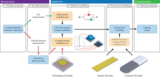
An overview of the major steps involved in creating and implementing multi-domain LED digital twins is described in detail by Martin et al. [3]. The steps are summarized in Figure 1 and briefly outlined here. First, a thermal-electrical-optical characterization of the physical LED device is performed (step 1). The testing protocols and methods are discussed in [4,5,6,7] and take the established testing standards JEDEC JESD51-14, JESD51-51, JESD51-52, and CIE 225:2017 [8,9,10,11] into account. The results of the characterization are so-called iso-thermal current-voltage-flux (IVL) characteristics and thermal transient characteristics of the LED device. This data will be reported in future standard LED electronic datasheets [12] (step 2).
Next, the multi-domain LED digital twin, also referred to as the LED multi-domain compact model (MDCM), is extracted from the characterization data (step 3). The LED MDCM consists of two parts. The first part is a chip-level multi-domain model. It calculates the forward voltage, power dissipation, radiant flux, and luminous flux from the forward current and junction temperature. Poppe et al. [13,14] discuss several sets of equations that can be used for this purpose. The extraction of the chip-level model is achieved by fitting the parameters of the equations to the IVL characteristics. The second part of the LED MDCM is a package-level compact thermal model (CTM). The LED CTM is a thermal RC-network attached to a simplified geometric representation of the LED. It calculates the relevant operating temperatures of the LED package, such as junction, phosphor and solder temperatures, from the power dissipation. The CTM extraction procedure is described by Bornoff et al. [15,16]. It involves the calibration of a detailed thermal model using the thermal transient characteristics, and the optimization of the RC-network to produce matching thermal dynamic behavior. In a fully realized LED digital twin, the two parts of the LED MDCM are coupled and solved self-consistently.
Finally, the LED digital twin is implemented in the larger system-level model of an LED-based lighting product, for example an LED module or an LED luminaire (step 4). There are different approaches to the system-level model. One option is to generate a compact thermal model of the LED module or LED luminaire. Poppe et al. [17] describe a method to create thermal network compact models for luminaires, which have subsequently been used in Spice-like luminaire simulations [3,18] and in an Excel spreadsheet application [3,19]. Alternatively, model order reduction could be used instead of thermal network compact models [20,21,22,23]. Another approach is to perform the LED module or LED luminaire simulations using the LED MDCM directly in a 3D computational fluid dynamics (CFD) model [3,24]. Ultimately, the LED module or LED luminaire model is used for virtual prototyping (step 5).
In this publication, we assess and compare the accuracy and computation time of 3D CFD system-level models equipped with LED CTMs and with LED detailed models. While this study does not include a multi-domain chip-level model, the LED thermal model is most demanding in terms of computation time in this case. First, an LED detailed model and an LED CTM are created according to the Delphi4LED methodology by performing a thermal characterization and LED-level modelling. The obtained LED thermal models are then implemented into 3D CFD software in the system-level model of two use cases: (1) an LED module-level model, and (2) an LED luminaire-level model. In previous research [24], we compared the computation time required to simulate an LED module-level model with up to 22 LEDs using LED detailed models and using LED CTMs. It showed that using the LED CTMs reduces the computation time by approximately a factor 10 for a steady-state, conduction only model. The novelty of this work is that the analysis is extended to the luminaire-level model. Typically, a LED luminaire contains several LED modules, and thus contains larger numbers of LEDs. Moreover, all methods of heat transport must be taken into account and their impact on the computation time is investigated.
2. Materials and Methods
The Delphi4LED approach as outlined Figure 1 is followed to create an LED detailed model and an LED CTM and to subsequently implement them in an LED module-level model and an LED luminaire-level model. The methods and processes of three of the involved steps are each described in a subsection. The first subsection briefly explains the test procedures used to obtain the required characterization data from physical LED samples (LED device testing). In the second subsection, the creation of the LED detailed model and the LED CTM are described (LED-level modelling). Finally, in the third subsection, the implementation of the LED detailed model and the LED CTM in the LED module-level model and the LED luminaire-level model is specified.
2.1. LED Device Testing
For the investigations, a phosphor-converted white high-power LED with a color rendering index (CRI) of 70 and correlated color temperature (CCT) of 4000 K is used. Four physical samples of the same type LED are each assembled on an insulated metal substrate (IMS) board for testing. Figure 2a shows the detailed 3D geometry of the LED sample placed on the test board. A cross-sectional view of the LED package geometry is provided in Figure 2b. The LED package and the test board together constitute the device under test (DUT).
The device under test is placed on a cold plate. Thermal paste is applied between the test board and the cold plate to provide good thermal contact, and the board is fixed in place with two screws. To ensure reproducibility a torque screwdriver used. Simultaneous radiometric measurements and thermal transient measurements, i.e., the temperature response to a power step, are performed using commercially available testing equipment (Simcenter T3ster and TeraLED) [13,25,26]. For these measurements a fixed cold plate temperature of is used. In these tests, the DUT is first operated at a (total) forward current of until steady-state is reached. Then a power step is applied by decreasing the current to a measurement current of . The measured emitted radiant flux is subtracted from the electrical power to obtain the total thermal dissipation . The thermal dissipation is then used to normalize the transient temperature to obtain the transient thermal impedance , as well as the corresponding structure function (SF) and differential structure function (DSF). This is the thermal characterization data needed for the LED CTM in the LED-level modelling step.
2.2. LED-Level Modelling
Generating an LED CTM, in the form of a thermal RC-network, from the thermal transient characterization data involves two parts. In the first part, a detailed thermal model of the LED package is created and calibrated using the characterization data as described in [15]. Then, in the second part, the calibrated LED detailed model is subsequently used to generate training data for the LED CTM. This training data consist of thermal responses under several different boundary conditions. The training data is used to optimize the RC-values of the LED CTM, such that the errors in thermal behavior compared to LED detailed model are minimized [16]. Finally, after the LED CTM is optimized, the achieved accuracy is validated by subjecting both the detailed model and CTM to several additional boundary conditions, which were not used in the training, and determining the errors.
2.2.1. LED Detailed Model
For the LED detailed model, geometrical information is required. The outer dimensions of the LED are provided by the manufacturer. However, in order to have a sufficiently accurate model, additional information is extracted from microscope images, e.g., the chip size and phosphor layer size. For other internal geometrical characteristics, generally not provided by suppliers, an educated guess is made. This is for instance done for the die attach thickness. Minor mismatches in those thicknesses are later compensated during the calibration process by adjusting the thermal conductivity values. The geometric model of the LED package and test board shown in Figure 2 is used in the calibration process.
In the detailed model, thermal loads are applied to the junction as well as to the phosphor layer. They are considered the main contributors to the total heat dissipation. Indeed, there may be other package losses resulting from trapped light due to total internal reflections. Recently, Alexeev et al. discussed the effects of secondary heat sources on thermal transient analysis in detail [27]. However, since losses related to trapped light are difficult to quantify and localize without elaborate optical modelling, only the junction and phosphor losses are considered in this study. Since only the total dissipation is known, the power split between the junction and phosphor is included in the calibration as an optimization parameter, together with the thermal conductivity values of the materials in the model.
The LED detailed model is calibrated by minimizing the errors between the modelled and measured responses and SFs. The model parameters are optimized to best match all four measured samples simultaneously. The calibration is performed using commercially available 3D CFD software (Simcenter Flotherm XT 2019.2).
To produce training data for the LED CTM, the calibrated LED detailed model is virtually taken off the test board and subjected to sets of different boundary conditions. This is done by applying uniform heat transfer coefficients (HTCs) to four selected peripheral faces: the bottom face of the anode solder pad, the bottom face of the cathode solder pad, the bottom face of the thermal solder pad, and the top face of the package/dome. The purpose of using multiple boundary conditions is to ensure that the extracted CTM will be boundary condition independent (BCI). The four sets of heat transfer coefficients that are used to generate the training data for the CTM are listed in Table 1. These HTCs training sets are chosen to represent practical operating environments of LEDs and are in the same range as the HTC sets used for the same purpose in [28]. The generated training data consists of the transient temperature profiles obtained for a power step . Here, the index i indicates the junction layer, the phosphor layer, and each of the four faces to which HTCs are applied. The index h indicates the each of the four HTC training sets. This data is exported from the CFD software.
2.2.2. LED CTM
A CTM, in the form of a thermal RC-network, is optimized to produce matching thermal behavior under the same boundary conditions, i.e., the four imposed HTC training sets. The chosen network topology is illustrated in Figure 3. Each node i of the thermal network has a thermal capacitance to ground. A line between two nodes m and n indicates that the nodes are connected by a thermal resistor . Compared to the network topology used in earlier studies [16,28], our network topology has an additional node between the junction and phosphor nodes (node 4), and between the phosphor and dome nodes (node 2). It was found by trial and error that those nodes are necessary to better fit the dynamic behavior, particularly of the phosphor and dome nodes.
The RC-network optimization is performed by code developed in Python and works in a manner similar to that described by Schweitzer [29]. It uses the derivative-free BOBYQA algorithm [30] implementation from the NLopt library [31]. An advantage of performing the optimization separately outside the CFD software is that stand-alone RC-network evaluations are faster, which means that several 10,000 to 100,000 optimization iterations can be made in a few minutes.
First, the training data is imported and the corresponding thermal (transfer) impedances are calculated. Subsequently, the RC-network is numerically solved for the same power step to obtain the CTM temperatures of nodes i under HTC training sets h. The corresponding thermal (transfer) impedances are again calculated as . By varying the and values, the difference in dynamic thermal behavior between the detailed model and the RC-network CTM is minimized using the following cost function:
where index h runs over all four HTC training sets, index i runs over the nodes included in the optimization, and index j runs over the time steps for which the simulation is performed. The included nodes are the junction, phosphor, and peripheral nodes, i.e., . In this particular case node 11 is not explicitly included due to symmetry.
To assess the accuracy and boundary condition independence of the optimized LED CTM, both the LED CTM and the LED detailed model are tested under twenty additional HTC sets. The twenty HTC testing sets are listed in Table 2. These sets are combinations generated using the design of experiments functionality of the CFD software. For each of the peripheral faces, the lower and upper HTC bounds were set to the minimum and maximum values that occur in the training sets. Since the HTC testing sets were not used to train the model, they provide a better evaluation of the predictive temperature accuracy of the LED CTM compared to the detailed model. In the report on end-user specifications of the Delphi4LED project [32] the required junction temperature accuracy is stated as 2%.
Finally, to be able to interface with a larger 3D system-level model, the LED CTM is attached to simplified 3D geometric representation of the LED package, as indicated in Figure 3. While the outer contours of the simplified geometry are identical to those of the detailed model, it has no internal structure. The faces of the simplified geometry that are connected to the peripheral nodes of the RC-network have the same surface area as the corresponding faces of the detailed model.
2.3. System-Level Modelling
Two use cases are investigated to assess the predicted junction temperature accuracy and computation time performance of the LED CTM, compared to the LED detailed model, integrated in a 3D system-level model: (1) an LED module-level model, and (2) an LED luminaire-level model. The thermal environment of the LED CTMs and the LED detailed models is now explicitly simulated in these cases, instead of imposed by uniform HTCs. Please note that both the LED module-level model and the luminaire-level model presented here are solely intended for the purpose of numerically assessing the LED CTM accuracy and performance, compared to the LED detailed model. They are by no means optimized for thermal management or any other actual product requirements.
While the described methods and models can in principle be used in any 3D CFD software, we used Simcenter Flotherm XT 2019.2. All reported computation times are obtained on a workstation laptop with an Intel Core i7-6820HQ ( GHz, 4 cores) processor. Unless stated otherwise, the default computational mesh settings (‘Standard Resolution’) of the software tool are used.
2.3.1. LED Module-Level Model
The LED module-level model consists of a simplified printed circuit board (PCB) populated with an array of LEDs, as illustrated in Figure 4. The board is 25 mm wide, 90 mm long and has a 1 mm thick dielectric layer (1 W/mK) and a 70 m thick copper layer ( 386 W/mK). Several LEDs, , are uniformly distributed on top of the copper layer. The number of LEDs along the x-axis is , and the number of LEDs along the y-axis is . For up to 15, a single row of LEDs is used (), for between 16 and 30, two rows of LEDs are used (), for between 31 and 45, three rows of LEDs are used (), and for greater than 45, four rows of LEDs are used (). The bottom face of the dielectric layer is kept at a fixed uniform temperature and only solid conduction is considered in this model.
2.3.2. LED Luminaire-Level Model
The LED luminaire model consists of a simplified luminaire housing and five instances of the LED module, as illustrated in Figure 5. Each of the LED modules has LEDs ( and ), resulting in total number of 60 LEDs. The luminaire housing is made of an aluminum alloy ( 140 W/mK) and has fins located above the LED modules for cooling to the surrounding air. In this luminaire-level model, conduction, convection and radiation are all taken into account, increasing the model complexity with flow simulation. All solid-fluid interfaces are assigned a surface emissivity of 0.8, including the anodized surface of the luminaire housing, and the ambient temperature is set at .
3. Results
In this section, the created LED-level models (detailed model and CTM) and the results of using the LED-level models in a system-level model (module and luminaire) are presented. The first part presents the results of the physical LED device testing. Then, the second part presents the modelling results at LED-level. It includes the calibration of the LED detailed model, and the extraction and validation of the LED CTM. Next, the third part presents the accuracy and performance results of the LED module-level model. Finally, the fourth part presents the accuracy and performance results of the LED-luminaire model.
3.1. LED Device Testing Results
Subtracting the measured radiant flux from the supplied electrical power results in the total dissipated thermal power of the DUT. It is found that . The reported uncertainty of W indicates the standard deviation between the four measured samples.
Figure 6 shows the transient behavior of the DUT obtained from the measurements. The thermal impedance is presented in Figure 6a. The corresponding structure functions (SF) and differential structure functions (DSF) are shown in Figure 6b. The four measured samples show good reproducibility. The largest relative deviation in measured between the four samples is about 4%, and occurs in the early transient (), where initial correction has to be applied due to electrical transients present in the measurement signal. The measured steady-state has a relative deviation of around . Using an additional `dry’ thermal transient additional measurement, i.e., without thermal paste applied between board and cold plate, the junction-to-board resistance was determined according to the standard JEDEC JESD51-14 [8]. The junction-to-board thermal resistance of the DUT is found as .
3.2. LED-Level Modelling Results
First, the model parameters of the detailed model, i.e., the thermal conductivity values of the materials and junction-phosphor power split, were calibrated to match the and SF of the measured LED devices. The power split in the detailed model that best fits the measurements was found in the calibration as approximately 77% in the junction and 23% in the phosphor. The , SF and DSF of the calibrated LED detailed model are shown together with those obtained from the measurements in Figure 6. Overall, the curves match well. Some deviations between the SFs and between the locations of the peaks and valleys of the DSFs are observed for approximately . However, since we are ultimately only interested in the LED package, without the board, no further improvements to matching this part of the SF are required.
Next, training data was generated using the calibrated LED detailed model for four HTC training sets. This training data was subsequently used to optimize the RC-values of the LED CTM. The optimized RC-values are given in Table 3. The column lists the thermal capacitance to ground for each of the nodes, and the array lists the thermal resistances between connected nodes of the RC-network. Since only the lower triangular entries are displayed.
The thermal transient behavior of the calibrated LED detailed model and the optimized RC-network LED CTM are compared for the four HTC training sets in Figure 7. The largest absolute error after optimization is about K/W and occurs between approximately and for the phosphor node in HTC training set 3. For steady-state conditions, the relative errors are all smaller than 2%, and smaller than 1% for the values corresponding to the junction. This results in junction temperatures that match within K for the training data.
The relative errors in steady-state temperature rise, , for the twenty HTC testing sets are plotted in Figure 8. The junction temperature errors range from about 0.6% to about 1.7%, remaining within the 2% requirement. All other temperature errors also remain within this limit, with the exception of the dome temperature for five of the twenty HTC testing sets. However, it should be noted that the temperature requirement is only specified for the junction temperature [32].
3.3. LED Module-Level Model
To assess the accuracy and performance of the LED CTM, compared to the LED detailed model, implemented in the LED module-level model, it was simulated with multiple numbers of LEDs. Since in each case the LEDs are uniformly distributed over the board, and the bottom face of the board is kept at a uniform temperature , the varies less than K between individual LEDs. For this reason only a single value, the average for all LEDs on the board, is reported for each case. The results are presented in Figure 9.
When there is only a small number of LEDs on the board, the distance between the individual LEDs is large enough that no mutual influence, or `cross-talk’, is experienced by the LEDs. This can be observed in the constant for up to 4 in Figure 9a. When the number of LEDs is further increased, gradually rises. As mentioned, between and , we change from a single row () to two rows () of LEDs. This results in an effective increase in the distance between individual LEDs and causes the drop in . This occurs again, albeit less pronounced, when the number of rows is increased to three () and to four ().
Comparing the average obtained using the LED CTM and the LED detailed model, the same behavior is observed. Nevertheless, the predictions of the LED CTM are systematically lower. The absolute difference in between the LED CTM and the LED detailed model decreases from about K for to about K for . This corresponds to relative errors in between 6.0% for and 2.2% for , as shown in Figure 9b.
Inspecting the peripheral faces of the thermal pad, anode pad and cathode pad, reveals discrepancies in the average surface temperatures and in the heat transfer distribution. For example, for the average surface temperature rise, , of the thermal pad and the total heat transfer through the thermal pad in the LED detailed model are K and W respectively, whereas in the LED CTM they are K and W respectively. For these differences are smaller, which results in a smaller junction temperature error. In this case the average surface temperature rise of the thermal pad and the total heat transfer through the thermal pad in the LED detailed models are K and W respectively, whereas in the LED CTMs they are K and W respectively. To ensure that the observed differences cannot be attributed to mesh convergence issues, the simulations for , , and were repeated with higher mesh density. The results were reproduced within K.
The time required by the central processor unit (CPU) to solve the model is shown as a function of the number of LEDs in Figure 10a. Up to 60 LEDs, the computation time increases approximately linearly for the LED CTMs, while the computation time using the LED detailed models increases super-linearly. The ratio between the CPU times using the LED detailed models and the LED CTMs is plotted in Figure 10b. It can be seen that for a single LED, using the CTM results in about a factor 2 reduction of computation time. For 60 LEDs the required computation time is reduced by nearly a factor 13 when the LED CTM is used instead of the LED detailed model. This is in line with our previous findings [24].
3.4. LED Luminaire-Level Model
In the LED luminaire-level model, the bottom faces of the LED modules are in direct thermal contact with the luminaire housing, instead of being kept at a constant fixed temperature. This results larger gradients in the board temperature, in particular for LED modules 3, 4 and 5. This is illustrated in the temperature plot presented in Figure 11. As a consequence, there are also larger variations in among LEDs on the same board than in the previous case of the LED module-level model. For this reason not only the average for each of the modules is reported, but also the minimum and maximum are listed in Table 4. Since the geometry of the model has a plane of symmetry, the values should be the same for LED module 1 and 2, and for LED module 3 and 5. The values obtained from the model are indeed very similar for these boards, apart from some small variations of K between LED module 1 and 2, which can be caused by asymmetries in the computational mesh.
As a general note, such high values indicate an improved thermal design would be necessary in practice. Comparing the values between the LED detailed models and the LED CTMs shows that the junction temperatures predicted by the LED CTMs are again systematically lower. The largest absolute error found in this case is K, which is in the same range as the errors found previously in the LED module-level model, and occurs for the LEDs with the largest on LED modules 3 and 5. The relative errors in range from about 0.3% to 1.1% in this case. Inspecting the average surface temperature rise of the thermal pad and the total heat transfer through the thermal pad of those LEDs again reveals similar discrepancies as before. For the detailed model they are K and W respectively, and for the CTM they are K and W respectively.
The LED luminaire-level model containing the LED detailed models took 9016 s to solve, whereas the model containing the LED CTMs only needed 2153 s, resulting in a reduction of a factor 4.2. This is smaller than the computation time reduction that was found for 60 LEDs in the LED module-level model. Besides that the luminaire-level model comprises a larger geometry than the module-level model, convection and radiation are also simulated in this case. To assess the impact of convection and radiation on the computation time, the simulation of the luminaire-level model with LED CTMs is repeated with convection and radiation each turned off separately. Without radiation the model is solved in 1907 s, and without convection the model is solved in 706 s.
4. Discussion
An RC-network LED CTM was successfully generated. The steady-state junction temperature error of the LED CTM, compared to the LED detailed model, was evaluated between 0.6% and 1.7% on LED-level under imposed uniform HTCs. This meets the requirement of 2% stated in the Delphi4LED end-users’ specifications [32].
A similar RC-network LED CTM, for a different LED package, is reported in [28]. The main differences are that a network topology with only nine instead of eleven nodes was used, the CTM was trained under three instead of four HTC training sets, using and a cost function based on the SF instead of . A slightly better relative error range of about 0.6% to 1.2% in the predicted steady-state junction temperature rise is reported there. Nevertheless, in both cases an acceptable accuracy for steady-state thermal behavior is achieved with an RC-network LED CTM. However, both in the present case and in [28] it appears more difficult to also achieve accurate dynamic behavior, in particular for the phosphor node. This indicates that further refinement of the extraction process or used network topology may still be necessary for cases in which the LED CTM is not operated in steady-state conditions. Another development in achieving accurate dynamic LED-level models that should be mentioned here is the BCI reduced order model (BCI-ROM) approach [20,21]. Recently, Bornoff and Gaal [28] compared this approach to the RC-network CTM and discussed its advantages related to extraction (no choices on a network topology have to be made) and accuracy (the required accuracy is prescribed by the user a priori for a wide range of HTCs). However, at the moment BCI-ROMs cannot be implemented yet in commercially available 3D CFD software.
When implemented in a 3D system-level, the LED CTM predicted slightly but systematically lower junction temperatures than the LED detailed model. The largest difference was K among the two studied use cases. Inspecting the peripheral faces of the thermal pad, anode pad and cathode pad, revealed discrepancies between the LED CTMs and LED detailed models in the average surface temperatures and in the heat transfer distribution. This is likely caused by the fact that the LED CTM is extracted under uniform peripheral conditions, whereas gradients exist in the more realistic 3D thermal environment. This situation could be improved by splitting the anode, cathode and thermal pad surfaces in multiple surfaces and assigning each their own node in the RC-network. However, this is at the cost of making the LED CTM more complex. The error could also be partly related to the choice and number of HTC training sets. In the original DELPHI project for semiconductor CTMs, 38 HTC sets were proposed, and later even larger sets were tested [33]. However, it was shown that smaller subsets of five HTCs can still lead to accurate CTMs [33,34]. The range of thermal operating environments that is relevant for LEDs is much smaller, but to date no studies have been performed involving the number and type of HTC sets to apply for accurate LED CTM extraction.
In the LED module-level model, absolute errors in of up to K and relative errors of up to 6.0% were found when comparing the model with LED CTMs and LED detailed models. In the LED luminaire-level model, absolute errors in of up to K and relative errors of up to 1.1% were found when comparing the model with LED CTMs and LED detailed models. While the absolute errors are on the same scale in both cases, the relative errors are substantially smaller in the luminaire-level case. This is explained by the larger total thermal resistance to ambient of the luminaire system, resulting in a larger temperature rise. Although the CTM meets the 2% error requirement compared to the detailed model on luminaire-level, in the LED module-level model the relative errors are larger. Hence the aforementioned potential improvements may be necessary, depending on the end-user’s needs. It should also be stressed however that we only considered the error of the extracted and implemented LED CTM compared to the LED detailed model. Compared to reality, for example if we were to measure a physical prototype, there may be various additional sources of errors. Some examples include: measurement uncertainties, uncertainties in the thermal dissipation of the components, and uncertainties related to the CFD simulation itself [35]. Additionally, the thermal resistance of the LED package may only represent a small fraction of the entire thermal resistance to ambient, especially at LED luminaire-level. When that is the case, the accuracy of the predicted compared to a physical prototype will also largely depend on the accuracy of the part of the model besides the LEDs.
Regarding the computation time, using the LED CTM in the LED module-level model resulted in a reduction from about a factor 2 with one LED up to almost a factor 13 with 60 LEDs. In the LED luminaire-level model with 60 LEDs, a reduction of about a factor 4 was achieved using the LED CTMs. Of course, the exact computation time will be different in every case and depends on the complexity of the luminaire design. The difference in the achieved reduction between the studied cases can be explained by the fact that the luminaire-level model has a larger 3D environment, more complex shapes, and that convection and radiation are considered. As a result, the LEDs themselves constitute a relatively smaller part of the entire model than in the case of the LED module-level model, and hence their relative impact on the total calculation time decreases. In particular, the flow simulations were found responsible for a large part of the computation time in the studied case. When turned off, the computation time decreased by about a factor 3, from 2153 s to 706 s. Without radiation, the computation time decreased by about 10%. Nevertheless, the factor 4 reduction for the simplified LED luminaire-level model is still significant when a large number of scenarios needs to be simulated in a design parameter optimization. Furthermore, the gains will increase significantly for higher LED counts, as demonstrated by the LED module-level model. As an example, this approach could therefore be highly advantageous when modelling systems containing LED filaments, as each filament may contain several hundreds of LEDs.
5. Conclusions and Outlook
To summarize, we created an LED detailed model and an LED CTM following the Delphi4LED methodology and assessed the accuracy and computation time of 3D CFD system-level models equipped with these LED models. Compared to previous work [24], the analysis was extended to luminaire-level. This involved including higher number of LEDs, up to 60, and taking all heat transfer mechanisms into account. The cases discussed in this work demonstrate that using Delphi4LED LED CTMs in digital luminaire designs can provide a significant reduction in computation time while maintaining the required accuracy compared to a LED detailed model.
With this approach, any node could be added to the LED model in order to monitor a thermally critical part of the LED. In this case, the temperature of the node of interest does need to be monitored during the LED testing. This way it can be included in the detailed model calibration in order to obtain an accurate model and predictions for this temperature. It would, for example, be interesting to do this for the phosphor temperature. While our LED CTM has a phosphor node, no phosphor temperatures were measured and accounted for in the calibration of the LED detailed model. Therefore, the modeled phosphor temperatures cannot currently be validated. In many cases, it is also not straightforward to monitor the temperature phosphor temperature. In the present case, the silicone dome covering the phosphor precludes measurements using thermocouples or infrared (IR) thermography. However, methods based on the spectral distribution of the converted light [36,37], or specifically prepared phosphors with magnetic nano-particles [38] could in principle be used.
Finally, the present study focused on 3D thermal modeling of the LED-based lighting designs using an RC-network LED CTM. It is expected that a future implementation of LED BCI-ROMs in 3D system-level models will provide an alternative option for the RC-network CTM. Additionally, only the LED CTM was considered. The implemented model will be extended in future work with a chip-level multi-domain model to obtain a fully realized LED digital twin. Another useful addition to the luminaire-level model is to include lifetime prediction [39], which will be the subject of a follow up paper.
Author Contributions
Conceptualization, G.M.; methodology, M.v.d.S. and G.M.; software, M.v.d.S.; validation, J.Y. and G.M.; formal analysis, M.v.d.S.; investigation, M.v.d.S.; resources, J.Y.; data curation, M.v.d.S.; writing–original draft preparation, M.v.d.S.; writing–review and editing, G.M. and J.Y.; visualization, M.v.d.S.; supervision, G.M.; project administration, G.M.; funding acquisition, G.M. All authors have read and agreed to the published version of the manuscript.
Funding
This research received no external funding.
Conflicts of Interest
The authors declare no conflict of interest.
Abbreviations
The following abbreviations are used:
| BCI | boundary condition independent |
| CCT | correlated color temperature |
| CFD | computational fluid dynamics |
| CPU | central processing unit |
| CRI | color rendering index |
| CTM | compact thermal model |
| DSF | differential structure function |
| DUT | device under test |
| HTC | heat transfer coefficient |
| IMS | insulated metal substrate |
| IR | infrared |
| LED | light-emitting diode |
| PCB | printed circuit board |
| MDCM | multi-domain compact model |
| ROM | reduced order model |
| SF | structure function |
References
- Delphi4LED Project Website. Available online: https://delphi4led.org (accessed on 27 March 2019).
- Bornoff, R.; Hildenbrand, V.; Lugten, S.; Martin, G.; Marty, C.; Poppe, A.; Rencz, M.; Schilders, W.H.; Yu, J. Delphi4LED—From measurements to standardized multi-domain compact models of LED: A new European R&D project for predictive and efficient multi-domain modeling and simulation of LEDs at all integration levels along the SSL supply chain. In Proceedings of the 2016 22nd International Workshop on Thermal Investigations of ICs and Systems (THERMINIC), Budapest, Hungary, 21–23 September 2016; pp. 174–180. [Google Scholar] [CrossRef]
- Martin, G.; Marty, C.; Bornoff, R.; Poppe, A.; Onushkin, G.; Rencz, M.; Yu, J. Luminaire Digital Design Flow with Multi-Domain Digital Twins of LEDs. Energies 2019, 12, 2389. [Google Scholar] [CrossRef] [Green Version]
- Bein, M.C.; Hegedus, J.; Hantos, G.; Gaal, L.; Farkas, G.; Rencz, M.; Poppe, A. Comparison of two alternative junction temperature setting methods aimed for thermal and optical testing of high power LEDs. In Proceedings of the 2017 23rd International Workshop on Thermal Investigations of ICs and Systems (THERMINIC), Amsterdam, The Netherlands, 27–29 September 2017; pp. 1–4. [Google Scholar] [CrossRef]
- Hantos, G.; Hegedus, J.; Bein, M.C.; Gaal, L.; Farkas, G.; Sarkany, Z.; Ress, S.; Poppe, A.; Rencz, M. Measurement issues in LED characterization for Delphi4LED style combined electrical-optical-thermal LED modeling. In Proceedings of the 2017 IEEE 19th Electronics Packaging Technology Conference (EPTC), Singapore, 6–9 December 2017; pp. 1–7. [Google Scholar] [CrossRef]
- Onushkin, G.A.; Bosschaart, K.J.; Yu, J.; van Aalderen, H.J.; Joly, J.; Martin, G.; Poppe, A. Assessment of isothermal electro-optical-thermal measurement procedures for LEDs. In Proceedings of the 2017 23rd International Workshop on Thermal Investigations of ICs and Systems (THERMINIC), Amsterdam, The Netherlands, 27–29 September 2017; pp. 1–6. [Google Scholar] [CrossRef]
- Farkas, G.; Gaal, L.; Bein, M.; Poppe, A.; Ress, S.; Rencz, M. LED Characterization Within the Delphi4LED Project. In Proceedings of the 2018 17th IEEE Intersociety Conference on Thermal and Thermomechanical Phenomena in Electronic Systems (ITherm), San Diego, CA, USA, 29 May–1 June 2018; pp. 262–270. [Google Scholar] [CrossRef]
- JEDEC JESD51-14: Transient Dual Interface Test Method for the Measurement of the Thermal Resistance Junction to Case of Semiconductor Devices with Heat Flow Trough a Single Path; Technical Report; JEDEC Solid State Technology Association: Arlington, VA, USA, 2010.
- JEDEC JESD51-51: Implementation of the Electrical Test Method for the Measurement of Real Thermal Resistance and Impedance of Light-Emitting Diodes with Exposed Cooling; Technical Report; JEDEC Solid State Technology Association: Arlington, VA, USA, 2012.
- JEDEC JESD51-52: Guidelines for Combining CIE 127-2007 Total Flux Measurements with Thermal Measurements of LEDs with Exposed Cooling Surface; Technical Report; JEDEC Solid State Technology Association: Arlington, VA, USA, 2012.
- Zong, Y.; Chou, P.; Dekker, P.; Distl, R.; Godo, K.; Hanselaer, P.; Heidel, G.; Hulett, J.; Oshima, K.; Poppe, A.; et al. CIE 225:2017 Optical Measurement of High-Power LEDs; Technical Report; International Commission on Illumination: Vienna, Austria, 2017. [Google Scholar] [CrossRef]
- Martin, G.; Marty, C.; Bornoff, R.; Vaumorin, E.; Kleij, A.; Onushkin, G.; Poppe, A. From Measurements to Standardised Multi-Domain Compact Models of LEDs using LED E-Datasheets. In Proceedings of the 29th Quadrennial Session of the CIE. International Commission on Illumination, Washington, DC, USA, 14–22 June 2019; CIE: Vienna, Austria, 2019; pp. 379–386. [Google Scholar] [CrossRef]
- Poppe, A. Multi-domain compact modeling of LEDs: An overview of models and experimental data. Microelectron. J. 2015, 46, 1138–1151. [Google Scholar] [CrossRef]
- Poppe, A.; Farkas, G.; Gaál, L.; Hantos, G.; Hegedüs, J.; Rencz, M. Multi-Domain Modelling of LEDs for Supporting Virtual Prototyping of Luminaires. Energies 2019, 12, 1909. [Google Scholar] [CrossRef] [Green Version]
- Bornoff, R.; Farkas, G.; Gaal, L.; Rencz, M.; Poppe, A. LED 3D thermal model calibration against measurement. In Proceedings of the 2018 19th International Conference on Thermal, Mechanical and Multi-Physics Simulation and Experiments in Microelectronics and Microsystems (EuroSimE), Toulouse, France, 15–18 April 2018; pp. 1–7. [Google Scholar] [CrossRef]
- Bornoff, R. Extraction of Boundary Condition Independent Dynamic Compact Thermal Models of LEDs—A Delphi4LED Methodology. Energies 2019, 12, 1628. [Google Scholar] [CrossRef] [Green Version]
- Poppe, A.; Hegedus, J.; Szalai, A.; Bornoff, R.; Dyson, J. Creating multi-port thermal network models of LED luminaires for application in system level multi-domain simulation using spice-like solvers. In Proceedings of the 2016 32nd Thermal Measurement, Modeling & Management Symposium (SEMI-THERM), San Jose, CA, USA, 14–17 March 2016; pp. 44–49. [Google Scholar] [CrossRef]
- Poppe, A. Simulation of LED based luminaires by using multi-domain compact models of LEDs and compact thermal models of their thermal environment. Microelectron. Reliab. 2017, 72, 65–74. [Google Scholar] [CrossRef]
- Marty, C.; Yu, J.; Martin, G.; Bornoff, R.; Poppe, A.; Fournier, D.; Fournier, D. Design flow for the development of optimized LED luminaires using multi-domain compact model simulations. In Proceedings of the 2018 24rd International Workshop on Thermal Investigations of ICs and Systems (THERMINIC), Stockholm, Sweden, 26–28 September 2018; pp. 1–7. [Google Scholar] [CrossRef]
- Codecasa, L. A novel approach for generating boundary condition independent compact dynamic thermal networks of packages. IEEE Trans. Components Packag. Technol. 2005, 28, 593–604. [Google Scholar] [CrossRef]
- Codecasa, L.; D’Alessandro, V.; Magnani, A.; Rinaldi, N.; Zampardi, P.J. Fast novel thermal analysis simulation tool for integrated circuits (FANTASTIC). In Proceedings of the THERMINIC 2014—20th International Workshop on Thermal Investigations of ICs and Systems, London, UK, 24–26 September 2014; Volume 2014, pp. 1–6. [Google Scholar] [CrossRef]
- Codecasa, L.; Magnani, A.; D’Alessandro, V.; Rinaldi, N.; Metzger, A.G.; Bornoff, R.; Parry, J. Novel MOR approach for extracting dynamic compact thermal models with massive numbers of heat sources. In Proceedings of the 2016 32nd Thermal Measurement, Modeling & Management Symposium (SEMI-THERM), San Jose, CA, USA, 14–17 March 2016; pp. 218–223. [Google Scholar] [CrossRef]
- Lungten, S.; Bornoff, R.; Dyson, J.; Maubach, J.M.L.; Schilders, W.H.A.; Warner, M. Dynamic compact thermal model extraction for LED packages using model order reduction techniques. In Proceedings of the 2017 23rd International Workshop on Thermal Investigations of ICs and Systems (THERMINIC), Amsterdam, The Netherlands, 27–29 September 2017; pp. 1–6. [Google Scholar] [CrossRef]
- Martin, G.; Yu, J.; Zuidema, P.; van der Schans, M. Luminaire Digital Design Flow with Delphi4LED LEDs Multi-Domain Compact Model. In Proceedings of the 2019 25th International Workshop on Thermal Investigations of ICs and Systems (THERMINIC), Lecco, Italy, 25–27 September 2019; Volume 2019, pp. 1–5. [Google Scholar] [CrossRef]
- Farkas, G.; Vader, Q.; Poppe, A.; Bognar, G. Thermal investigation of high power Optical Devices by transient testing. IEEE Trans. Components Packag. Technol. 2005, 28, 45–50. [Google Scholar] [CrossRef]
- Farkas, G.; Hara, T.; Rencz, M. Thermal transient testing. In Wide Bandgap Power Semiconductor Packaging; Elsevier: Amsterdam, The Netherlands, 2018; pp. 127–153. [Google Scholar] [CrossRef]
- Alexeev, A.; Onushkin, G.; Linnartz, J.P.; Martin, G. Multiple Heat Source Thermal Modeling and Transient Analysis of LEDs. Energies 2019, 12, 1860. [Google Scholar] [CrossRef] [Green Version]
- Bornoff, R.; Gaal, L. Comparison of Model Order Reduction and Thermal Network Approaches in the Extraction of Dynamic Compact Thermal Models of LEDs. In Proceedings of the 2019 25th International Workshop on Thermal Investigations of ICs and Systems (THERMINIC), Lecco, Italy, 25–27 September 2019; Volume 2019, pp. 1–7. [Google Scholar] [CrossRef]
- Schweitzer, D. Generation of multisource dynamic compact thermal models by RC-network optimization. In Proceedings of the 29th IEEE Semiconductor Thermal Measurement and Management Symposium, San Jose, CA, USA, 17–21 March 2013; pp. 116–123. [Google Scholar] [CrossRef]
- Powell, M.J.D. The BOBYQA Algorithm for Bound Constrained Optimization without Derivatives (NA2009/06); Technical Report; Department of Applied Mathematics and Theoretical Physics, University of Cambridge: Cambridge, UK, 2009. [Google Scholar]
- Johnson, S.G. The NLopt Nonlinear-Optimization Package. Available online: http://github.com/stevengj/nlopt (accessed on 28 January 2020).
- Lungten, S.; Alexeev, A.; Onushkin, G. Delphi4LED D1.1—Report on End-User Specifications. Available online: https://delphi4led.org/pydio/public/b610a0 (accessed on 15 April 2019).
- Lasance, C.J.M. Ten Years of Boundary-Condition- Independent Compact Thermal Modeling of Electronic Parts: A Review. Heat Transf. Eng. 2008, 29, 149–168. [Google Scholar] [CrossRef]
- Lasance, C.; Den Hertog, D.; Stehouwer, P. Creation and evaluation of compact models for thermal characterisation using dedicated optimisation software. In Proceedings of the Fifteenth Annual IEEE Semiconductor Thermal Measurement and Management Symposium, San Diego, CA, USA, 9–11 March 1999; pp. 189–200. [Google Scholar] [CrossRef]
- Lasance, C.J. The conceivable accuracy of experimental and numerical thermal analyses of electronic systems. IEEE Trans. Components Packag. Technol. 2002, 25, 366–382. [Google Scholar] [CrossRef]
- Kusama, H.; Sovers, O.J.; Yoshioka, T. Line Shift Method for Phosphor Temperature Measurements. Jpn. J. Appl. Phys. 1976, 15, 2349–2358. [Google Scholar] [CrossRef]
- Yang, T.H.; Huang, H.Y.; Sun, C.C.; Glorieux, B.; Lee, X.H.; Yu, Y.W.; Chung, T.Y. Noncontact and instant detection of phosphor temperature in phosphor-converted white LEDs. Sci. Rep. 2018, 8, 296. [Google Scholar] [CrossRef] [PubMed]
- Du, Z.; Sun, Y.; Su, R.; Wei, K.; Gan, Y.; Ye, N.; Zou, C.; Liu, W. The phosphor temperature measurement of white light-emitting diodes based on magnetic nanoparticle thermometer. Rev. Sci. Instruments 2018, 89, 94901. [Google Scholar] [CrossRef] [PubMed]
- Hegedüs, J.; Hantos, G.; Poppe, A. Lifetime Modelling Issues of Power Light Emitting Diodes. Energies 2020, 13, 3370. [Google Scholar] [CrossRef]
Figure 1.
The Delphi4LED approach to creating and implementing LED digital twins (multi-domain compact models). The involved steps are indicated from top to bottom. Adapted from [3].
Figure 1.
The Delphi4LED approach to creating and implementing LED digital twins (multi-domain compact models). The involved steps are indicated from top to bottom. Adapted from [3].

Figure 2.
Detailed geometry of the LED under investigation: (a) The LED package assembled on the test board (DUT). (b) Cross-sectional view of the LED package geometry.
Figure 2.
Detailed geometry of the LED under investigation: (a) The LED package assembled on the test board (DUT). (b) Cross-sectional view of the LED package geometry.

Figure 3.
RC-network topology of the LED CTM (left), and two isometric views of the simplified 3D geometry of the LED CTM (right). The red arrows indicate to which surfaces (in blue) the temperatures of the peripheral nodes of the RC-network model are connected.
Figure 3.
RC-network topology of the LED CTM (left), and two isometric views of the simplified 3D geometry of the LED CTM (right). The red arrows indicate to which surfaces (in blue) the temperatures of the peripheral nodes of the RC-network model are connected.

Figure 4.
The LED module-level model. On the left an example is shown with LED detailed models ( and ), and on the right an example is shown with LED CTMs ( and ).
Figure 4.
The LED module-level model. On the left an example is shown with LED detailed models ( and ), and on the right an example is shown with LED CTMs ( and ).

Figure 5.
The LED luminaire-level model. On the left, the top part of the luminaire housing with cooling fins is visible, and on the right, the bottom part of the luminaire housing is visible, which supports five LED modules each with 12 LEDs ( and ). The rectangular outlines indicate the computational domain.

Figure 6.
Thermal transient characteristics of the measured LED device and the calibrated LED detailed model: (a) Thermal transient impedance of the DUT and calibrated detailed model. (b) Structure function and differential structure function of the DUT and the calibrated detailed model.
Figure 6.
Thermal transient characteristics of the measured LED device and the calibrated LED detailed model: (a) Thermal transient impedance of the DUT and calibrated detailed model. (b) Structure function and differential structure function of the DUT and the calibrated detailed model.

Figure 7.
Transient behavior of the LED detailed model (blue) and optimized LED CTM (red) for (a) HTC training set 1, (b) HTC training set 2, (c) HTC training set 3, and (d) HTC training set 4. The numbers correspond to the nodes of the RC-network: 1-dome, 3-phosphor, 5-junction, 9-thermal pad, and 10-dome.

Figure 8.
Relative errors in the steady-state of the LED CTM, compared to the LED detailed model, for each of the twenty HTC testing sets. The dashed line indicates the 2% junction temperature error requirement of the Delphi4LED end-user specifications [32].
Figure 8.
Relative errors in the steady-state of the LED CTM, compared to the LED detailed model, for each of the twenty HTC testing sets. The dashed line indicates the 2% junction temperature error requirement of the Delphi4LED end-user specifications [32].

Figure 9.
Average junction temperature rise of the LEDs in the LED module-level model: (a) comparison between the LED detailed model and the LED CTM, and (b) the relative error in the LED CTM values for different number of LEDs.
Figure 9.
Average junction temperature rise of the LEDs in the LED module-level model: (a) comparison between the LED detailed model and the LED CTM, and (b) the relative error in the LED CTM values for different number of LEDs.

Figure 10.
Time required to solve the LED module-level model: (a) comparison of CPU time between the LED detailed model and the LED CTM, and (b) the ratio in CPU time between the LED detailed model and the LED CTM.
Figure 10.
Time required to solve the LED module-level model: (a) comparison of CPU time between the LED detailed model and the LED CTM, and (b) the ratio in CPU time between the LED detailed model and the LED CTM.

Figure 11.
Surface temperature of the LED luminaire-level model with LED detailed models (top) and LED CTMs (bottom). For the LED CTMs, the temperature of the internal junction node is plotted on the LED geometry.
Figure 11.
Surface temperature of the LED luminaire-level model with LED detailed models (top) and LED CTMs (bottom). For the LED CTMs, the temperature of the internal junction node is plotted on the LED geometry.


Table 1.
HTC training sets used to generate training data for the LED CTM optimization.
| Set | HTC | ||
|---|---|---|---|
| Anode/Cathode Pad | Thermal Pad | Dome | |
| 1 | 10,000 | 25,000 | 10 |
| 2 | 3000 | 75,000 | 20 |
| 3 | 1500 | 20,000 | 100 |
| 4 | 50,000 | 10,000 | 5 |
Table 2.
HTC testing sets used to generate test data for the LED CTM validation.
| Set | HTC | ||
|---|---|---|---|
| Anode/Cathode Pad | Thermal Pad | Dome | |
| 1 | 42,725 | 13,250 | 66.75 |
| 2 | 1500 | 58,750 | 71.5 |
| 3 | 18,475 | 49,000 | 100 |
| 4 | 37,875 | 36,000 | 95.25 |
| 5 | 50,000 | 45,750 | 62 |
| 6 | 20,900 | 71,750 | 76.25 |
| 7 | 40,300 | 65,250 | 90.5 |
| 8 | 30,600 | 32,750 | 5 |
| 9 | 28,175 | 10,000 | 33.5 |
| 10 | 47,575 | 23,000 | 28.75 |
| 11 | 23,325 | 19,750 | 81 |
| 12 | 16,050 | 42,500 | 57.25 |
| 13 | 8775 | 16,500 | 47.75 |
| 14 | 35,450 | 68,500 | 52.5 |
| 15 | 6350 | 52,250 | 24 |
| 16 | 33,025 | 39,250 | 43 |
| 17 | 13,625 | 75,000 | 38.25 |
| 18 | 45,150 | 55,500 | 19.25 |
| 19 | 25,750 | 62,000 | 14.5 |
| 20 | 3925 | 29,500 | 85.75 |
Table 3.
Optimized thermal capacitance values and thermal resistance values of the LED CTM.
| C () | R () | |||||||||||
|---|---|---|---|---|---|---|---|---|---|---|---|---|
| Node | 1 | 2 | 3 | 4 | 5 | 6 | 7 | 8 | 9 | 10 | 11 | |
| 1 | 8.533 × 10⁻⁴ | |||||||||||
| 2 | 9.906 × 10⁻³ | 222.6 | ||||||||||
| 3 | 1.157 × 10⁻⁴ | 291.4 | ||||||||||
| 4 | 2.793 × 10⁻⁴ | 7.707 | ||||||||||
| 5 | 5.306 × 10⁻⁵ | 8.563 | ||||||||||
| 6 | 2.365 × 10⁻⁴ | 0.299 | ||||||||||
| 7 | 2.567 × 10⁻³ | 1.350 | ||||||||||
| 8 | 9.209 × 10⁻³ | 0.096 | ||||||||||
| 9 | 1.113 × 10⁻⁴ | 1268 | 1.822 | |||||||||
| 10 | 4.374 × 10⁻⁴ | 1645 | 4.911 | |||||||||
| 11 | 4.374 × 10⁻⁴ | 1645 | 4.911 | |||||||||
Table 4.
Minimum, average, and maximum junction temperature rises and relative errors for each of LED modules in the LED luminaire-level model.
Table 4.
Minimum, average, and maximum junction temperature rises and relative errors for each of LED modules in the LED luminaire-level model.
| LED Module | (K) | Rel. Error (%) | |||||||
|---|---|---|---|---|---|---|---|---|---|
| Detailed Model | CTM | ||||||||
| Min. | Avg. | Max. | Min. | Avg. | Max. | Min. | Avg. | Max. | |
| 1 | 118.8 | 121.1 | 122.2 | 118.2 | 120.3 | 121.7 | 0.4 | 0.7 | 0.9 |
| 2 | 118.9 | 121.1 | 122.2 | 118.3 | 120.3 | 121.6 | 0.5 | 0.7 | 0.9 |
| 3 | 100.7 | 113.2 | 120.7 | 99.8 | 112.2 | 119.4 | 0.5 | 0.9 | 1.1 |
| 4 | 101.5 | 114.3 | 121.8 | 100.8 | 113.6 | 120.7 | 0.3 | 0.7 | 0.9 |
| 5 | 100.7 | 113.2 | 120.7 | 99.8 | 112.2 | 119.4 | 0.5 | 0.9 | 1.1 |
© 2020 by the authors. Licensee MDPI, Basel, Switzerland. This article is an open access article distributed under the terms and conditions of the Creative Commons Attribution (CC BY) license (http://creativecommons.org/licenses/by/4.0/).
Share and Cite
MDPI and ACS Style
van der Schans, M.; Yu, J.; Martin, G. Digital Luminaire Design Using LED Digital Twins—Accuracy and Reduced Computation Time: A Delphi4LED Methodology. Energies 2020, 13, 4979. https://0-doi-org.brum.beds.ac.uk/10.3390/en13184979
AMA Style
van der Schans M, Yu J, Martin G. Digital Luminaire Design Using LED Digital Twins—Accuracy and Reduced Computation Time: A Delphi4LED Methodology. Energies. 2020; 13(18):4979. https://0-doi-org.brum.beds.ac.uk/10.3390/en13184979
Chicago/Turabian Stylevan der Schans, Marc, Joan Yu, and Genevieve Martin. 2020. "Digital Luminaire Design Using LED Digital Twins—Accuracy and Reduced Computation Time: A Delphi4LED Methodology" Energies 13, no. 18: 4979. https://0-doi-org.brum.beds.ac.uk/10.3390/en13184979
Note that from the first issue of 2016, this journal uses article numbers instead of page numbers. See further details here.