
Traffic, Air Pollution, Minority and Socio-Economic Status: Addressing Inequities in Exposure and Risk

Abstract
:
1. Introduction
2. Experimental Section
3. Results and Discussion
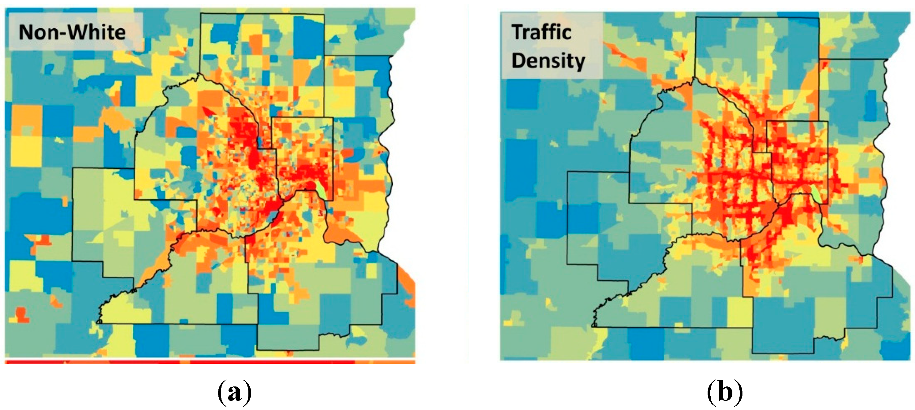
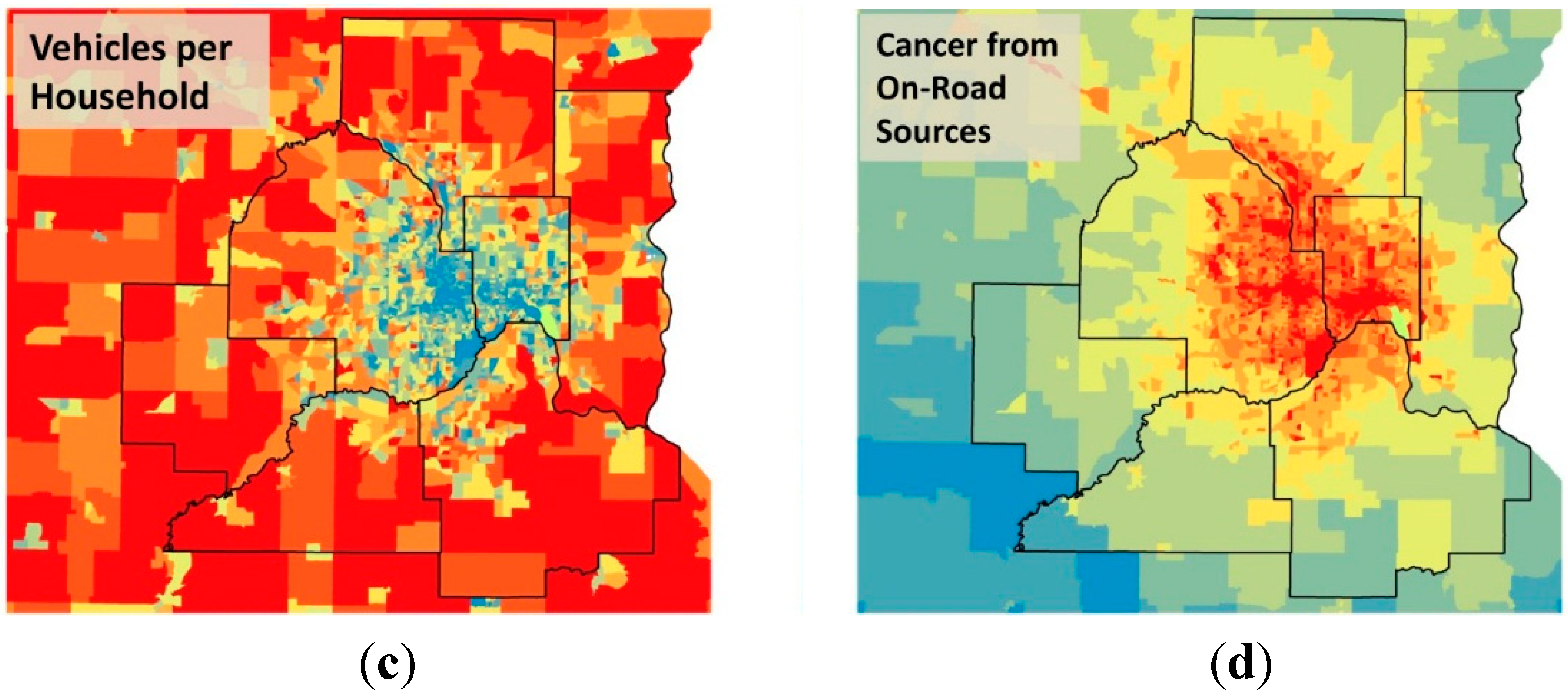
3.1. Study Area

| Demographic | Metro | Non-Metro | State |
|---|---|---|---|
| Block Groups | 2085 | 2026 | 4111 |
| Total Population | 2,807,902 | 2,434,012 | 5,241,914 |
| Asian | 173,813 | 29,255 | 203,068 |
| Black | 221,266 | 32,027 | 253,293 |
| Hispanic | 156,071 | 77,645 | 233,716 |
| American Indian | 16,109 | 36,098 | 52,207 |
| NonWhite | 636,174 | 208,899 | 845,073 |
| White | 2,171,728 | 2,225,113 | 4,396,841 |
| Less than High School | 136,915 | 162,331 | 299,246 |
| Bachelors Degree | 488,704 | 247,716 | 736,420 |
| House Value > $250K | 365,283 | 164,770 | 530,053 |
| Owner Occupied Housing | 790,821 | 757,306 | 1,548,127 |
| Rent < $700 | 84,010 | 113,370 | 197,380 |
| Rent > 30% Income | 152,194 | 94,975 | 247,169 |
| Rental Housing | 319,896 | 217,894 | 537,790 |
| >1 Vehicles in Household | 662,678 | 651,681 | 1,314,359 |
| Commute by Walk/Transit | 112,334 | 59,116 | 171,450 |
| Drove Alone | 1,138,275 | 942,865 | 2,081,140 |
| No Vehicles in Household | 87,946 | 56,296 | 144,242 |
| Below 100% of Poverty | 276,096 | 266,037 | 542,133 |
| Below 150% of Poverty | 448,882 | 461,489 | 910,371 |
| HH Income > $60K | 829,383 | 642,501 | 1,471,884 |
| Children Under 10 | 383,234 | 315,404 | 698,638 |
| Over 65 | 292,138 | 366,025 | 658,163 |
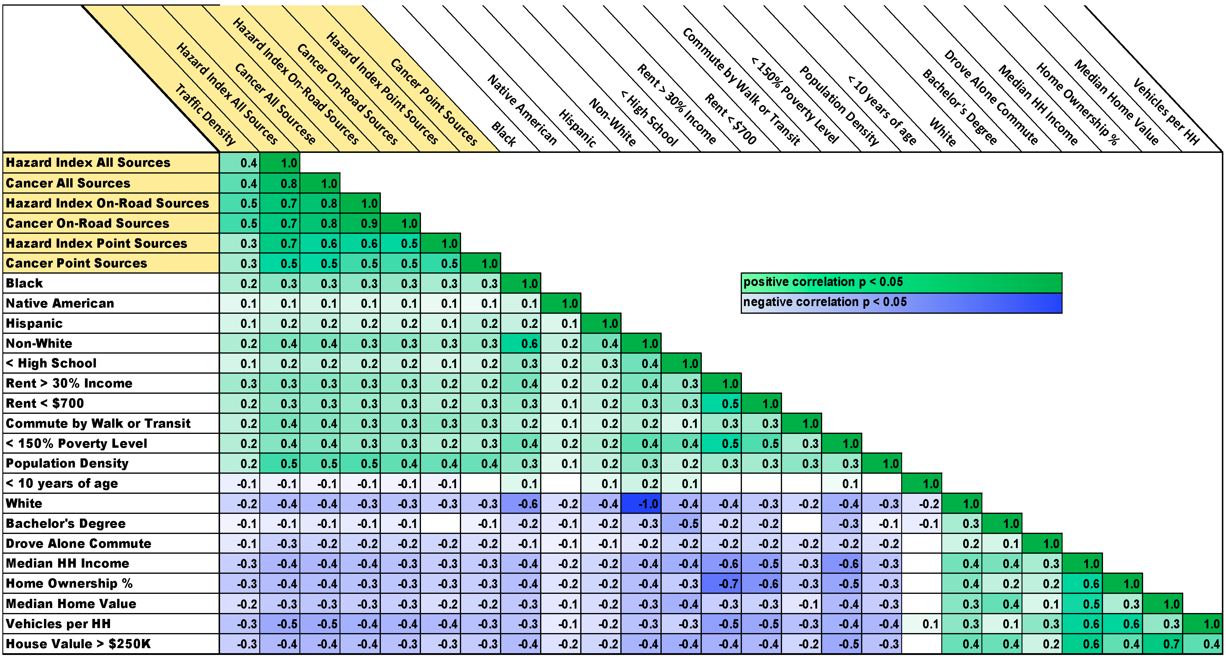
3.2. Correlations


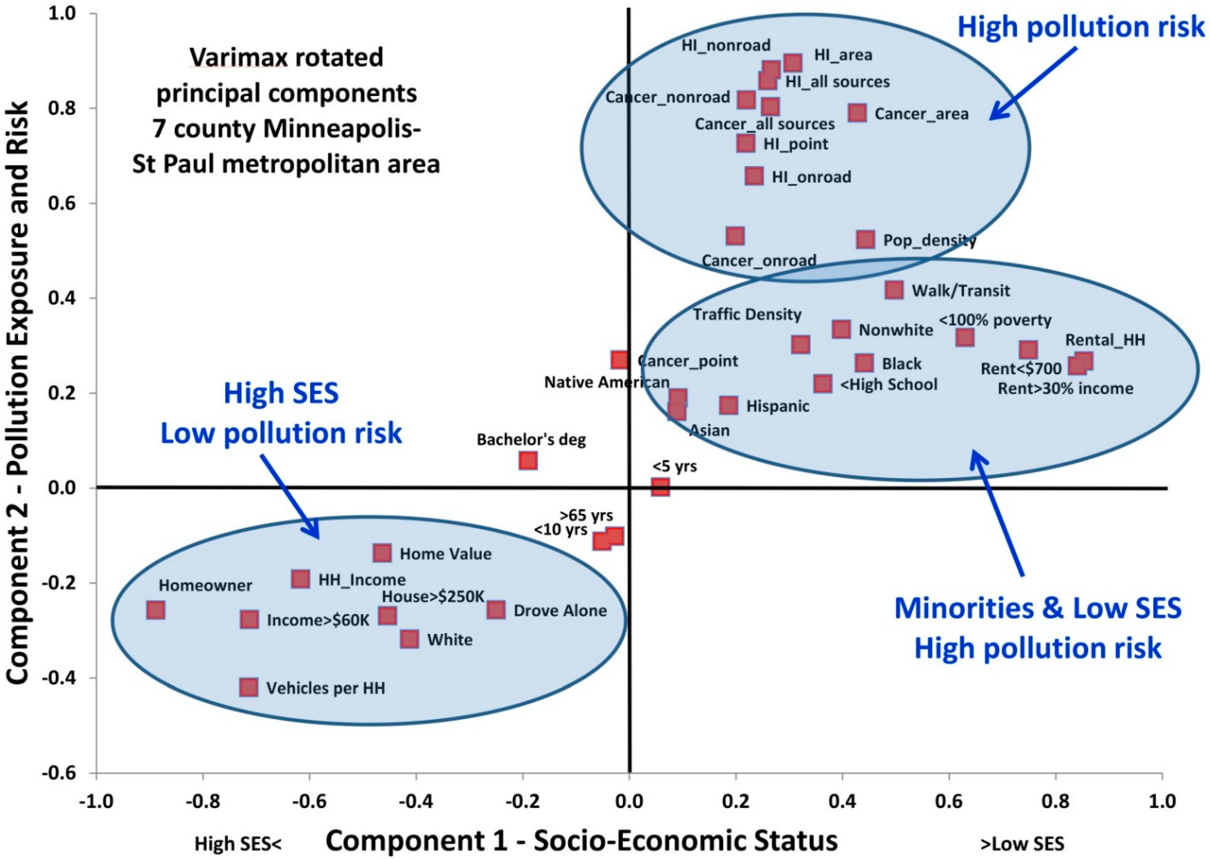
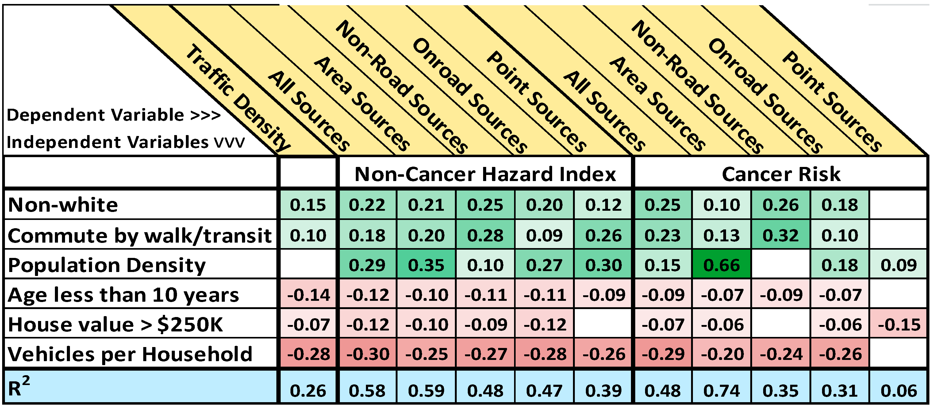
3.3. Regressions and Insights into Relationships

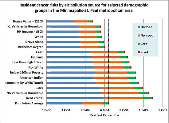
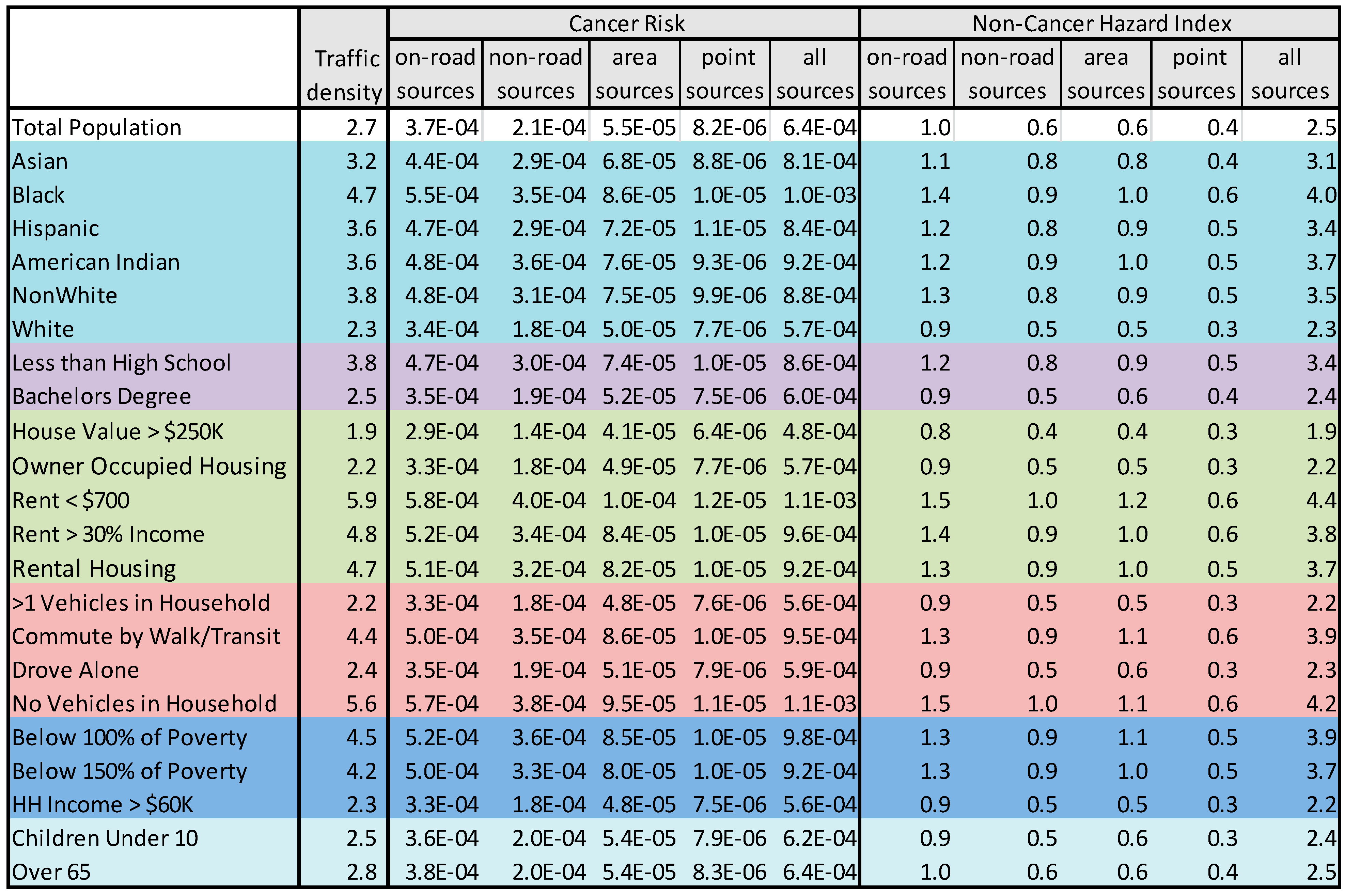
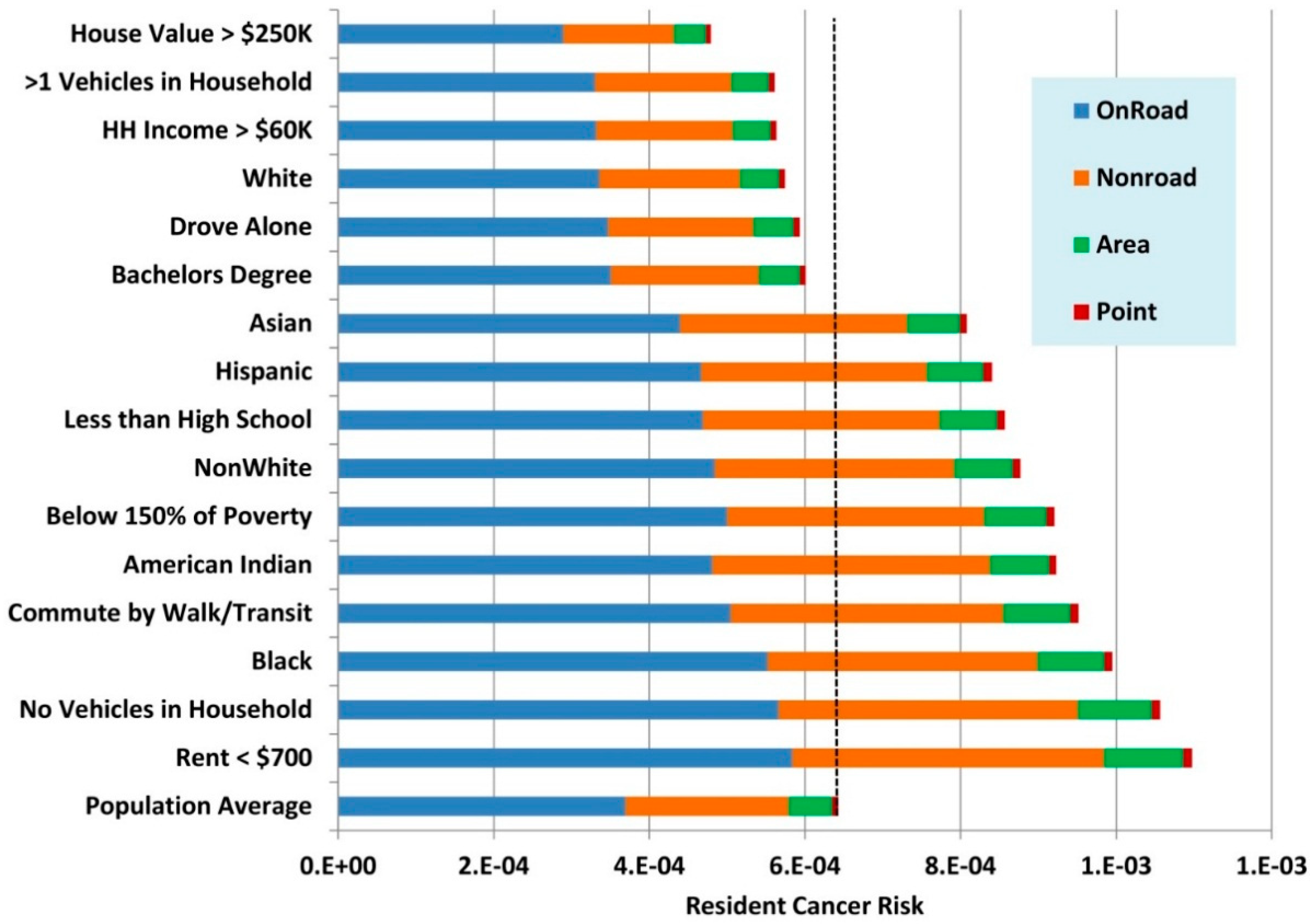
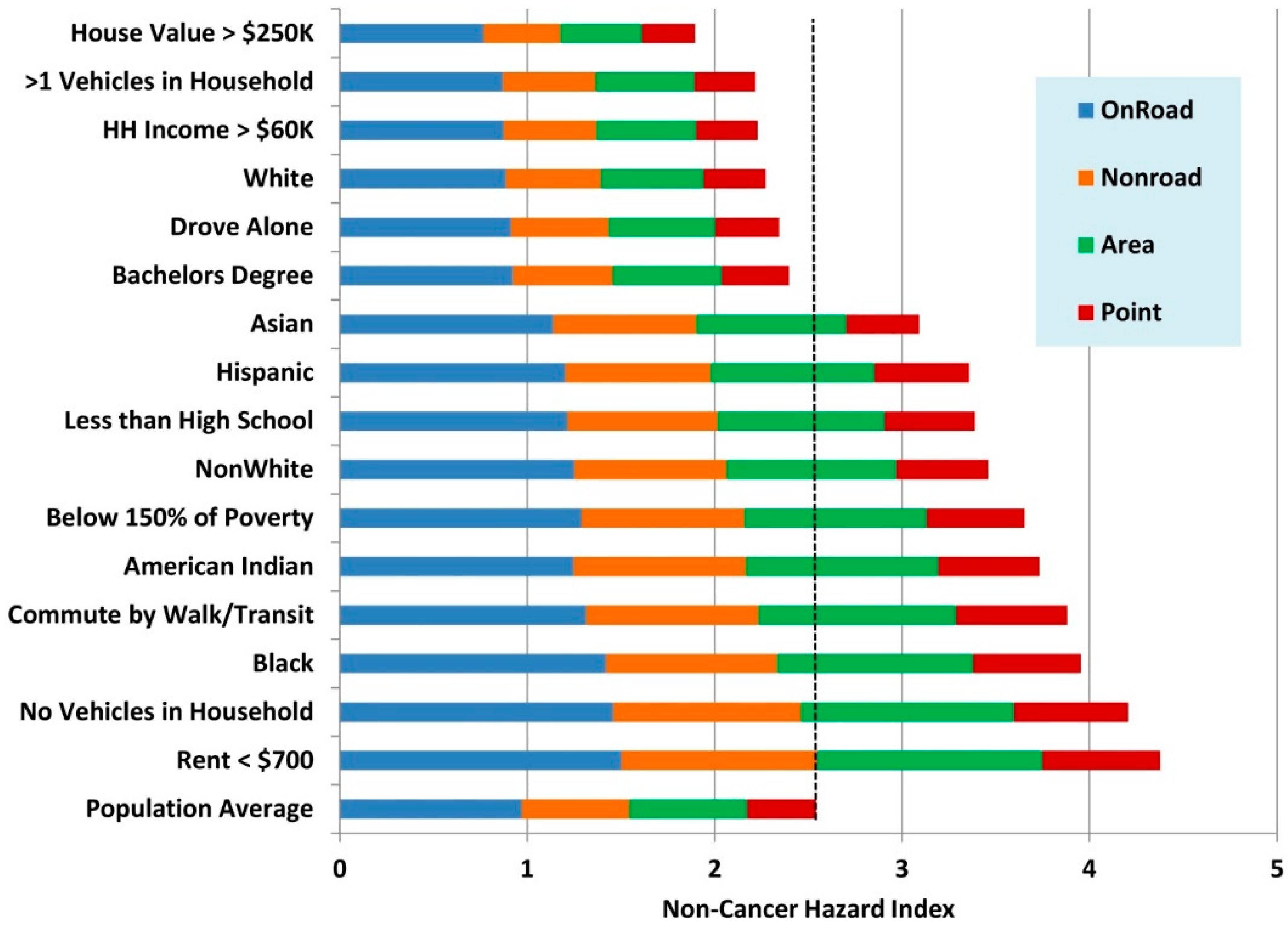
3.4. Risks by Demography and Air Pollution Source Category


3.5. Policy Implications
3.6. Limitations
4. Conclusions
Supplementary Files
Supplementary File 1Acknowledgments
Author Contributions
Conflicts of Interest
References
- Winkelstein, W.J.; Kantor, S.; Davis, E.W.; Maneri, C.S.; Mosher, W.E. The relationship of air pollution and economic status to total mortality and selected respiratory system mortality in men. Arch. Environ. Health 1967, 14, 162–171. [Google Scholar] [CrossRef] [PubMed]
- Bell, M.L.; Ebisu, K. Environmental inequality in exposures to airborne particulate matter components in the United States. Environ. Health Perspect. 2012, 120, 1699–1704. [Google Scholar] [PubMed]
- Evans, G.W. The environment of childhood poverty. Am. Psychol. 2004, 59, 77–92. [Google Scholar] [CrossRef] [PubMed]
- Evans, G.W.; Kantrowitz, E. Socioeconomic status and health: The potential role of environmental risk exposure. Annu. Rev. Public Health 2002, 23, 303–331. [Google Scholar] [CrossRef] [PubMed]
- Havard, S.; Zmirou-navier, D.; Schillinger, C.; Bard, D. Traffic-related air pollution and socioeconomic status. Epidemiology 2009, 20, 223–230. [Google Scholar] [CrossRef] [PubMed]
- Marshall, J.D.; Swor, K.R.; Nguyen, N.P. Prioritizing environmental justice and equality: Diesel emissions in Southern California. Environ. Sci. Technol. 2014, 48, 4063–4068. [Google Scholar] [CrossRef] [PubMed]
- Matte, T.D.; Ross, Z.; Kheirbek, I.; Eisl, H.; Johnson, S.; Gorczynski, J.E.; Kass, D.; Markowitz, S.; Pezeshki, G.; Clougherty, J.E. Monitoring intraurban spatial patterns of multiple combustion air pollutants in New York City: Design and implementation. J. Expo. Anal. Environ. Epidemiol. 2013, 23, 223–231. [Google Scholar] [CrossRef]
- Rowangould, G.M. A census of the US near-roadway population: Public health and environmental justice considerations. Transp. Res. Part D Transp. Environ. 2013, 25, 59–67. [Google Scholar] [CrossRef]
- Woodruff, T.J.; Parker, J.D.; Kyle, A.D.; Schoendorf, K.C. Disparities in exposure to air pollution during pregnancy. Environ. Health Perspect. 2003, 111, 942–946. [Google Scholar] [CrossRef] [PubMed]
- Young, G.S.; Fox, M.A.; Trush, M.; Kanarek, N.; Glass, T.A. Differential exposure to hazardous air pollution in the United States: A multilevel analysis of urbanization and neighborhood socioeconomic deprivation. Int. J. Environ. Res. Public Health 2012, 9, 2204–2225. [Google Scholar] [CrossRef] [PubMed]
- USEPA National Center for Environmental Assessment EPA/600/R-99/060. Sociodemographic Data Used for Identifying Potentially Highly Exposed Populations. 1999. Available online: http://webapp1.dlib.indiana.edu/virtual_disk_library/index.cgi/5269549/FID678/HEP/hep.pdf (accessed on 14 April 2015).
- Hajat, A.; Diez-Roux, A.V.; Adar, S.D.; Auchincloss, A.H.; Lovasi, G.S.; O’Neill, M.S.; Sheppard, L.; Kaufman, J.D. Air pollution and individual and neighborhood socioeconomic status: Evidence from the Multi-Ethnic Study of Atherosclerosis (MESA). Environ Health Perspect. 2013, 121, 1325–1333. [Google Scholar] [PubMed]
- Hao, Y.; Flowers, H.; Monti, M.M.; Qualters, J.R. U.S. census unit population exposures to ambient air pollutants. Int. J. Health Geogr. 2012, 11, 1–9. [Google Scholar] [CrossRef] [PubMed]
- Tian, N.; Xue, J.; Barzyk, T.M. Evaluating socioeconomic and racial differences in traffic-related metrics in the United States using a GIS approach. J. Expo. Sci. Environ. Epidemiol. 2013, 23, 215–222. [Google Scholar] [CrossRef] [PubMed]
- Clark, L.P.; Millet, D.B.; Marshall, J.D. National patterns in environmental injustice and inequality: Outdoor NO2 air pollution in the United States. PLoS One 2014, 9. [Google Scholar] [CrossRef] [PubMed]
- Basagaña, X.; Sunyer, J.; Kogevinas, M.; Zock, J.; Duran-Tauleria, E.; Jarvis, D.; Burney, P.; Anti, J.M.; European Community Respiratory Health Survey. Socioeconomic status and asthma prevalence in young adults the European Community Respiratory Health Survey. Am. J. Epidemiol. 2004, 160, 178–188. [Google Scholar] [CrossRef] [PubMed]
- Finkelstein, M.M.; Jerrett, M.; Deluca, P.; Finkelstein, N.; Verma, D.K.; Chapman, K.; Sears, M.R. Relation between income, air pollution and mortality: A cohort study. Can. Med. Assoc. J. 2003, 169, 1–6. [Google Scholar]
- Forastiere, F.; Stafoggiam, Ã.M.; Tasco, C.; Picciotto, S.; Agabiti, N.; Cesaroni, G.; Perucci, C.A. Socioeconomic status, particulate air pollution, and daily mortality: Differential exposure or differential susceptibility. Am. J. Ind. Med. 2007, 50, 208–216. [Google Scholar] [CrossRef] [PubMed]
- Gauderman, W.J.; Avol, E.; Lurmann, F.; Kuenzli, N.; Gilliland, F. Childhood asthma and exposure to traffic and nitrogen dioxide. Epidemiology 2005, 16, 12–15. [Google Scholar] [CrossRef] [PubMed]
- Gauderman, W.J.; Vora, H.; McConnell, R.; Berhane, K.; Gilliland, F.; Thomas, D.; Lurmann, F.; Avol, E.; Kunzli, N.; Jerrett, M.; et al. Effect of exposure to traffic on lung development from 10 to 18 years of age: A cohort study. Lancet 2007, 369, 571–577. [Google Scholar]
- Gwynn, R.C.; Thurston, G.D. The burden of air pollution: Impacts among racial minorities. Environ. Health Perspect. 2001, 109, 501–506. [Google Scholar] [CrossRef] [PubMed]
- Jerrett, M.; Burnett, R.T.; Ma, R.; Iii, C.A.P.; Krewski, D.; Newbold, K.B.; Thurston, G.; Shi, Y.; Finkelstein, N.; Calle, E.E.; et al. Spatial analysis of air pollution and mortality in Los Angeles. Epidemiology 2005, 16, 727–736. [Google Scholar] [CrossRef] [PubMed]
- Kariisa, M.; Foraker, R.; Buckley, T.; Pennell, M.; Diaz, P.; Wilkins, J.R. Differential ambient air pollution exposure in a chronic obstructive pulmonary disease cohort: The role of area-level socioeconomic factors. Environ. Justice 2014, 7, 18–26. [Google Scholar] [CrossRef]
- Kim, J.J.; Smorodinsky, S.; Lipsett, M.; Singer, B.C.; Hodgson, A.T.; Ostro, B. Traffic-related air pollution near busy roads: The east bay children’s respiratory health study. Am. J. Respir. Crit. Care Med. 2004, 170, 520–526. [Google Scholar] [CrossRef] [PubMed]
- Laurent, O.; Bard, D.; Filleul, L.; Segala, C. Effect of socioeconomic status on the relationship between atmospheric pollution and mortality. J. Epidemiol. Community Health 2007, 61, 665–675. [Google Scholar] [CrossRef] [PubMed]
- Lee, J.; Son, J.; Kim, H.; Kim, S. Effect of air pollution on asthma-related hospital admissions for children by socioeconomic status associated with area of residence. Arch. Environ. Occup. Health 2006, 61, 123–130. [Google Scholar] [CrossRef] [PubMed]
- Lipfert, F.W. Air pollution and poverty: Does the sword cut both ways? J. Epidemiol. Community Health 2004, 58, 2–3. [Google Scholar] [CrossRef] [PubMed]
- Martins, M.; Fatigati, F.; Vespoli, T.C.; Martins, L.; Pereira, L.A.; Martins, M.A.; Saldiva, P.H.; Braqa, A.L. Influence of socioeconomic conditions on air pollution adverse health effects in elderly people: An analysis of six regions in Sao Paulo, Brazil. J. Epidemiol. Community Health 2004, 58, 41–46. [Google Scholar] [CrossRef] [PubMed]
- Nandi, A.; Glymour, M.M.; Subramanian, S.V. Association among socioeconomic status, health behaviors, and all-cause mortality in the United States. Epidemiology 2014, 25, 170–177. [Google Scholar] [CrossRef] [PubMed]
- Newman, N.C.; Ryan, P.H.; Huang, B.; Beck, A.F.; Sauers, H.S.; Kahn, R.S. Traffic-related air pollution and asthma hospital readmission in children: A longitudinal cohort study. J. Pediatr. 2014, 5, 1–8. [Google Scholar]
- Pardo-Crespo, M.R.; Narla, N.P.; Williams, A.R.; Beebe, T.J.; Sloan, J.; Yawn, B.P.; Wheeler, P.H.; Juhn, Y.J. Comparison of individual-level versus area-level socioeconomic measures in assessing health outcomes of children in Olmsted County, Minnesota. J. Epidemiol. Community Health 2013, 67, 305–310. [Google Scholar] [CrossRef] [PubMed]
- Ponce, N.A.; Hoggatt, K.J.; Wilhelm, M.; Ritz, B. Preterm birth: The interaction of traffic-related air pollution with economic hardship in Los Angeles neighborhoods. Am. J. Epidemiol. 2005, 162, 140–148. [Google Scholar] [CrossRef] [PubMed]
- Pope, C.A.I.; Ezzati, M.; Dockery, D. Fine-particulate air pollution and life expectancy in the United States. N. Engl. J. Med. 2009, 360, 376–386. [Google Scholar] [CrossRef] [PubMed]
- Samet, J.; White, R. Urban air pollution, health, and equity. J. Epidemiol. Community Health 2004, 58, 3–5. [Google Scholar] [CrossRef] [PubMed]
- Schikowski, T.; Sugiri, D.; Ranft, U.; Gehring, U.; Heinrich, J.; Wichmann, H.-E.; Kramer, U. Long-term air pollution exposure and living close to busy roads are associated with COPD in women. Respir. Res. 2005, 6. [Google Scholar] [CrossRef]
- Wheeler, B.W.; Ben-Shlomo, Y. Environmental equity, air quality, socioeconomic status, and respiratory health: A linkage analysis of routine data from the Health Survey for England. J. Epidemiol. Community Health 2005, 59, 948–954. [Google Scholar] [CrossRef] [PubMed]
- Kim, J.J.; Huen, K.; Adams, S.; Smorodinsky, S.; Hoats, A.; Malig, B.; Lipsett, M.; Ostro, B. Residential traffic and children’s respiratory health. Environ. Health Perspect. 2008, 116, 1274–1279. [Google Scholar] [CrossRef] [PubMed]
- Smart Growth America. Measuring Sprawl 2014. Available online: http://www.smartgrowthamerica.org/documents/measuring-sprawl-2014.pdf (accessed on 27 January 2015).
- Transit for Livable Communities. Highway Lane Miles Per Capita, 2004. Available online: http://www.tlcminnesota.org/pdf/lanemilespercapita.pdf (accessed on 27 January 2015).
- Roberson, L. Where Sit Happens. Available online: http://www.menshealth.com/health/most-active-cities (accessed on 27 January 2015).
- Bicycling Magazine. America’s Top 50 Bike-Friendly Cities. Available online: http://www.bicycling.com/rides/best-cities/america-s-top-50-bike-friendly-cities (accessed on 27 January 2015).
- The Minnesota Compass Project, 2015. Available online: http://www.mncompass.org/ (accessed on 19 March 2015).
- The Minneapolis Foundation, 2013, oneMinneapolis, A Vision for Our City’s Success, 2013 Community Indicators Report. Available online: http://www.minneapolisfoundation.org/Libraries/Documents_for_Website/2013OneMinneapolisReport.sflb.ashx (accessed on 19 March 2015).
- Pratt, G.C.; Parson, K.; Shinoda, N.; Lindgren, P.; Dunlap, S.; Yawn, B.; Wollan, P.; Johnson, J. Quantifying traffic exposure. J. Expo. Sci. Environ. Epidemiol. 2013, 24, 1–7. [Google Scholar]
- Pratt, G.C.; Dymond, M.; Ellickson, K.; Thé, J. Validation of a novel air toxic risk model with air monitoring. Risk Anal. 2012, 32, 96–112. [Google Scholar] [CrossRef] [PubMed]
- US EPA. Human Health Risk Assessment Protocol for Hazardous Waste Combustion Facilities. 2005. Available online: http://www.epa.gov/osw/hazard/tsd/td/combust/risk.htm#hhrad (accessed on 27 January 2015). [Google Scholar]
- Morello-Frosch, R.; Pastor, M.; Sadd, J. Environmental justice and Southern California’s “Riskscape”: The distribution of air toxics exposures and health risks among diverse communities. Urban Aff. Rev. 2001, 36, 551–578. [Google Scholar] [CrossRef]
- Perlin, S.A.; Setzer, R.W.; Creason, J.; Sexton, K. Distribution of industrial air emissions by income and race in the United States: An approach using the Toxic Release Inventory. Environ. Sci. Technol. 1996, 29, 69–80. [Google Scholar] [CrossRef]
- Neumann, C.M.; Forman, D.L.; Rothlein, J.E. Hazard screening of chemical releases and environmental equity analysis of populations proximate to toxic release inventory facilities in Oregon. Environ. Health Perspect. 1998, 106, 217–226. [Google Scholar] [CrossRef] [PubMed]
- Perlin, S.A.; Wong, D.; Sexton, K. Residential proximity to industrial sources of air pollution: Interrelationships among race, poverty, and age. J. Air Waste Manag. Assoc. 2001, 51, 406–421. [Google Scholar] [CrossRef] [PubMed]
- Glaeser, E.L.; Kahn, M.E.; Rappaport, J. Why do the poor live in cities? The role of public transportation. J. Urban Econ. 2008, 63, 1–24. [Google Scholar] [CrossRef]
- U.S. Census Bureau. Small Area Income and Poverty Estimates; Quantifying Uncertainty in State and County Estimates. Available online: http://www.census.gov/did/www/saipe/methods/statecountyuncertainty.html (accessed on 27 January 2015).
- Williams, J.D. The 2010 Decennial Census: Background and Issues. 2011. Available online: http://www.census.gov/history/pdf/2010-background-crs.pdf (accessed on 27 January 2015). [Google Scholar]
- Batterman, S.; Chambliss, S.; Isakov, V. Spatial resolution requirements for traffic-related air pollutant exposure evaluations. Atmos. Environ. 2014, 94, 518–528. [Google Scholar] [CrossRef]
- Health Effects Institute. Advanced Collaborative Emissions Study (ACES): Lifetime Cancer and Non-Cancer Assessment in Rats Exposed to New Technology Diesel Exhaust. 2015. Available online: http://pubs.healtheffects.org/getfile.php?u=1039 (accessed on 14 April 2015).
© 2015 by the authors; licensee MDPI, Basel, Switzerland. This article is an open access article distributed under the terms and conditions of the Creative Commons Attribution license (http://creativecommons.org/licenses/by/4.0/).
Share and Cite
Pratt, G.C.; Vadali, M.L.; Kvale, D.L.; Ellickson, K.M. Traffic, Air Pollution, Minority and Socio-Economic Status: Addressing Inequities in Exposure and Risk. Int. J. Environ. Res. Public Health 2015, 12, 5355-5372. https://0-doi-org.brum.beds.ac.uk/10.3390/ijerph120505355
Pratt GC, Vadali ML, Kvale DL, Ellickson KM. Traffic, Air Pollution, Minority and Socio-Economic Status: Addressing Inequities in Exposure and Risk. International Journal of Environmental Research and Public Health. 2015; 12(5):5355-5372. https://0-doi-org.brum.beds.ac.uk/10.3390/ijerph120505355
Chicago/Turabian StylePratt, Gregory C., Monika L. Vadali, Dorian L. Kvale, and Kristie M. Ellickson. 2015. "Traffic, Air Pollution, Minority and Socio-Economic Status: Addressing Inequities in Exposure and Risk" International Journal of Environmental Research and Public Health 12, no. 5: 5355-5372. https://0-doi-org.brum.beds.ac.uk/10.3390/ijerph120505355