Reliability Analysis and Optimization of a Reconfigurable Matching Network for Communication and Sensing Antennas in Dynamic Environments through Gaussian Process Regression

 , , , ,
  , , and
Abstract
:1. Introduction
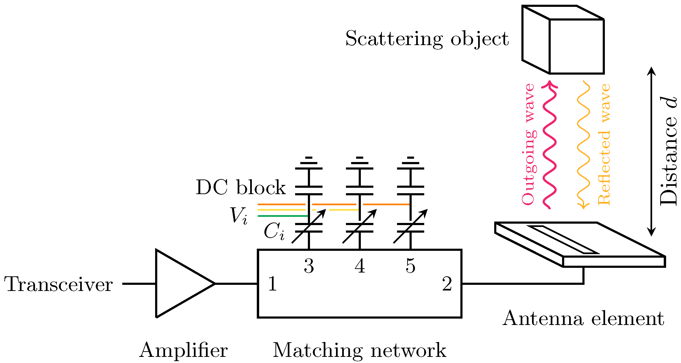
2. Setup
2.1. Matching Network
2.2. Antenna Element
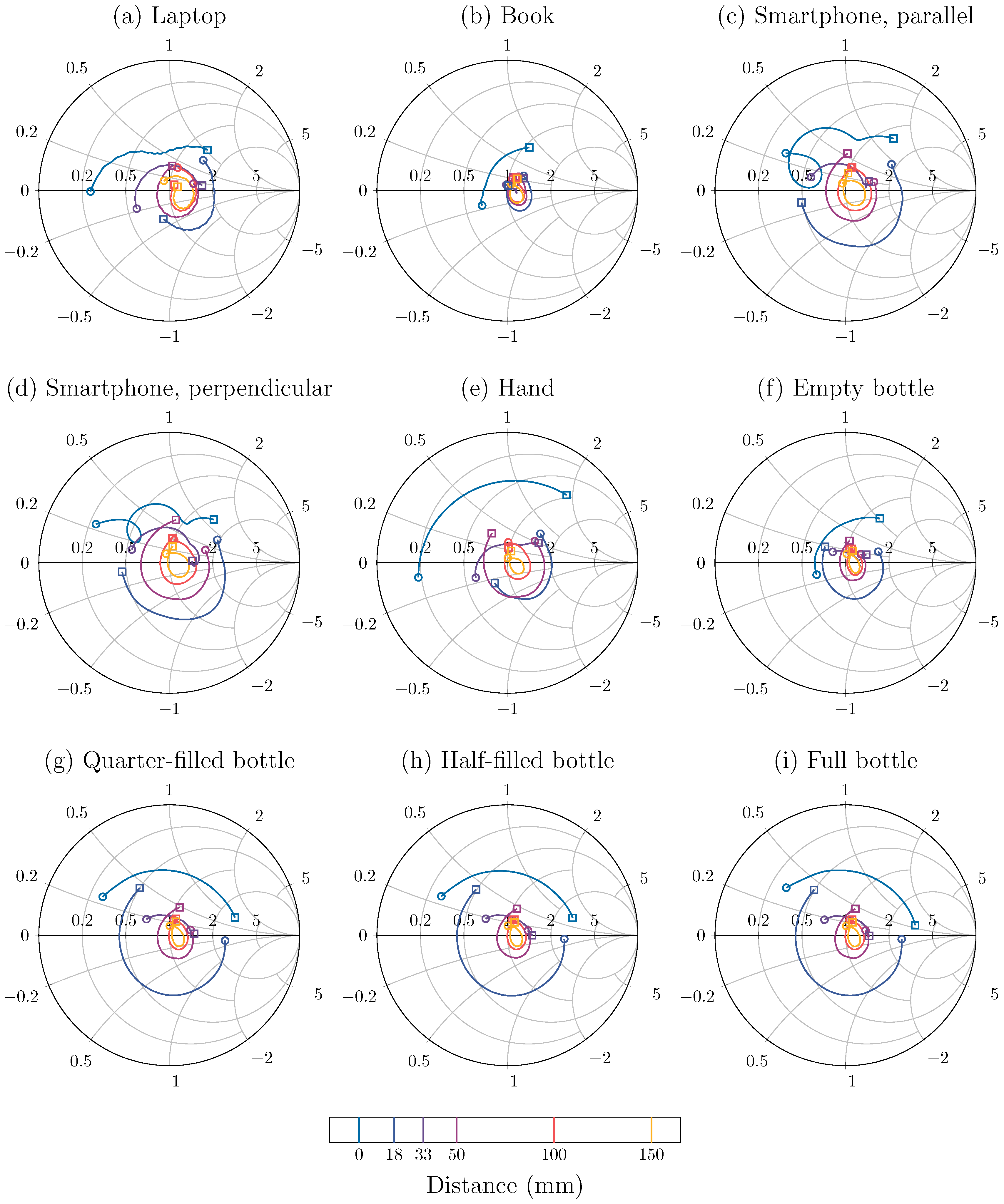
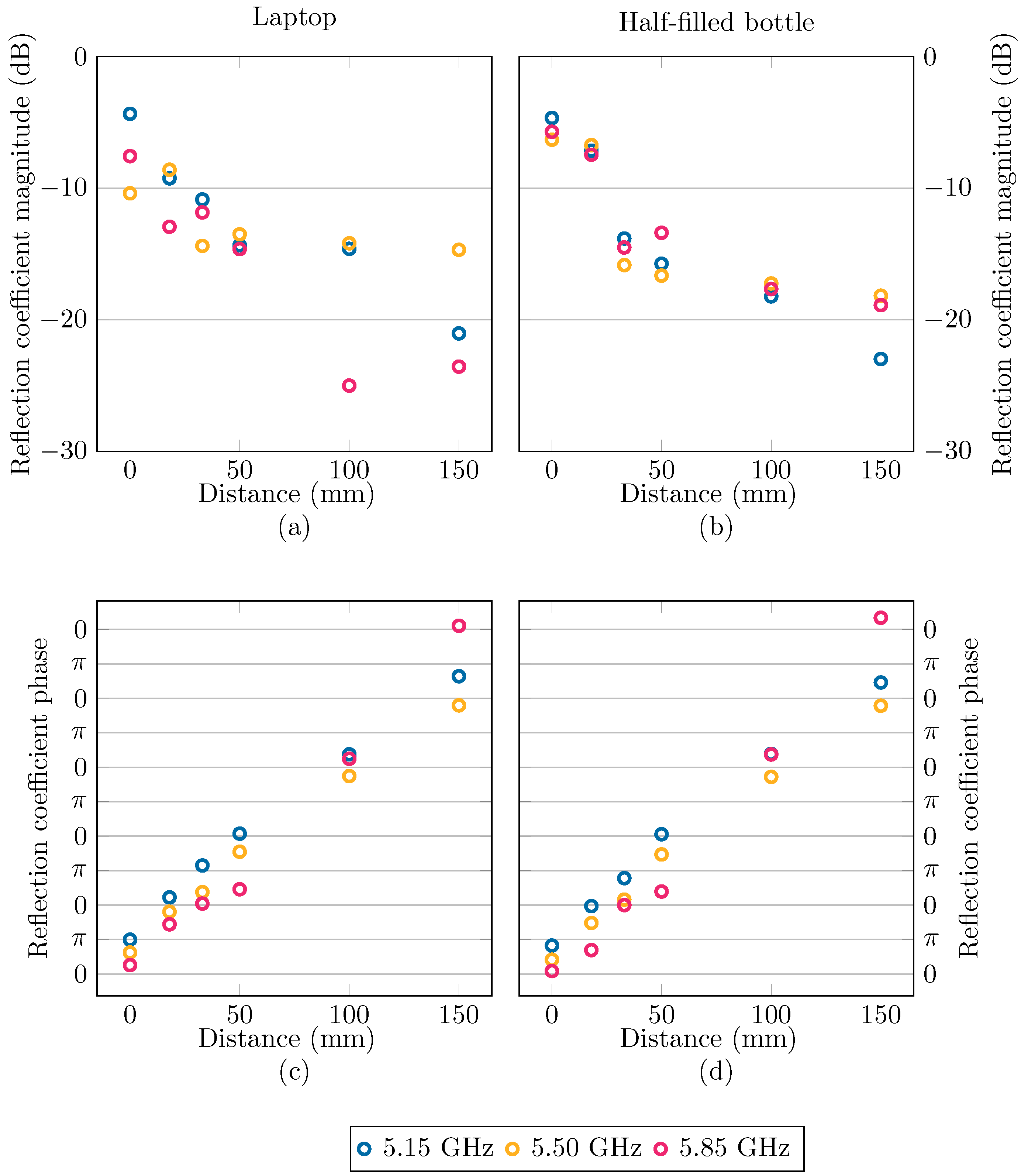
2.3. Experimental Setup and Results
3. Method
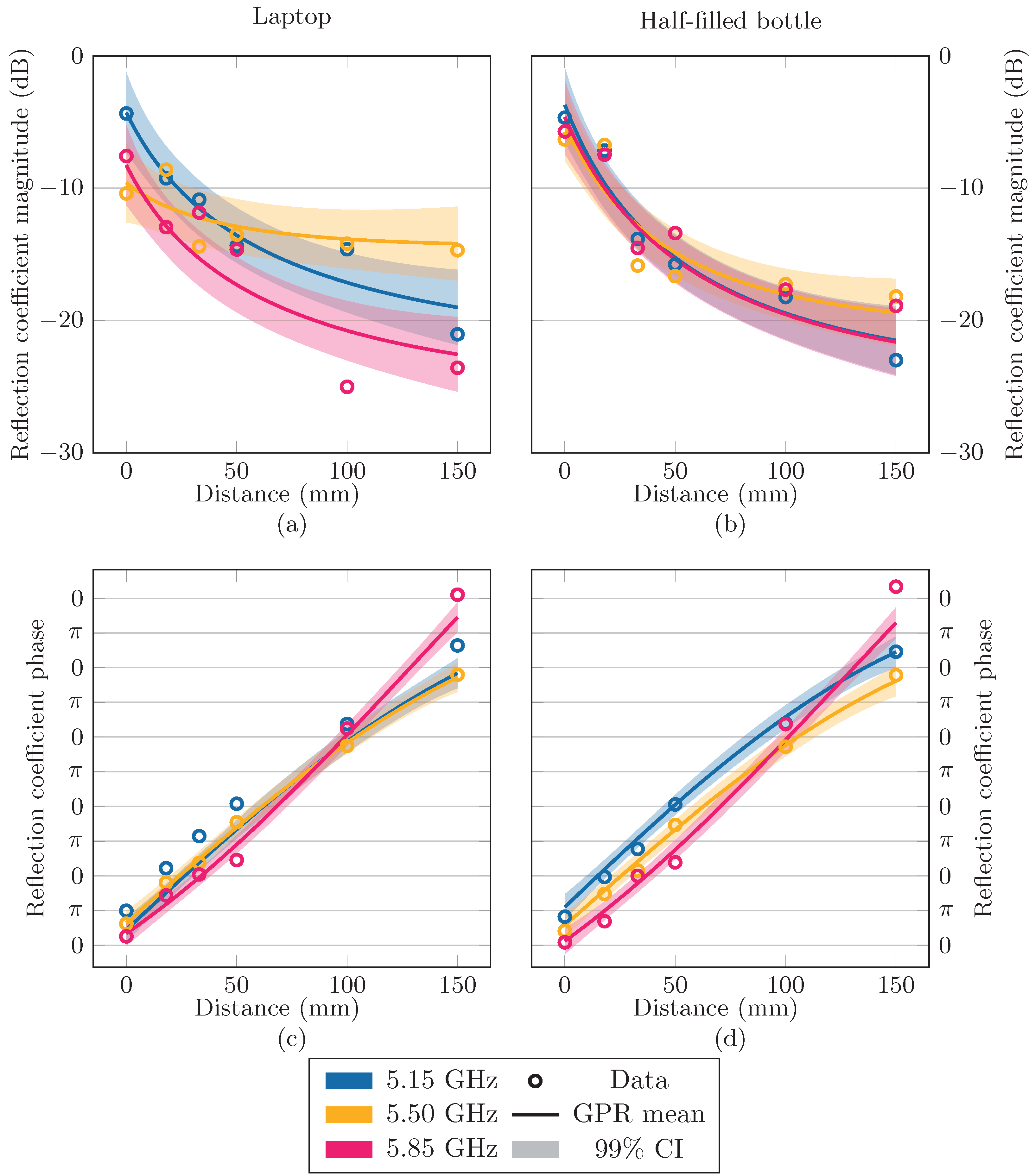
3.1. Gaussian Process Regression
3.2. Reliability Optimization
4. Application
5. Results
5.1. Impact of the Dynamic Environment
5.2. Improvements to Proposed Strategy
6. Conclusions
Author Contributions
Funding
Institutional Review Board Statement
Informed Consent Statement
Data Availability Statement
Conflicts of Interest
References
- Kopetz, H.; Steiner, W. Internet of things. In Real-Time Systems: Design Principles for Distributed Embedded Applications; Springer: Berlin/Heidelberg, Germany, 2022; pp. 325–341. [Google Scholar]
- Nguyen, D.C.; Ding, M.; Pathirana, P.N.; Seneviratne, A.; Li, J.; Niyato, D.; Dobre, O.; Poor, H.V. 6G Internet of Things: A comprehensive survey. IEEE Internet Things J. 2022, 9, 359–383. [Google Scholar] [CrossRef]
- Qiu, T.; Chen, N.; Li, K.; Atiquzzaman, M.; Zhao, W. How can heterogeneous internet of things build our future: A survey. IEEE Commun. Surv. Tutorials 2018, 20, 2011–2027. [Google Scholar] [CrossRef]
- Cirillo, F.; Wu, F.J.; Solmaz, G.; Kovacs, E. Embracing the future internet of things. Sensors 2019, 19, 351. [Google Scholar] [CrossRef]
- Bajic, B.; Rikalovic, A.; Suzic, N.; Piuri, V. Industry 4.0 implementation challenges and opportunities: A managerial perspective. IEEE Syst. J. 2020, 15, 546–559. [Google Scholar] [CrossRef]
- Majid, M.; Habib, S.; Javed, A.R.; Rizwan, M.; Srivastava, G.; Gadekallu, T.R.; Lin, J.C.W. Applications of wireless sensor networks and internet of things frameworks in the industry revolution 4.0: A systematic literature review. Sensors 2022, 22, 2087. [Google Scholar] [CrossRef]
- Silverio-Fernández, M.; Renukappa, S.; Suresh, S. What is a smart device-a conceptualisation within the paradigm of the internet of things. Vis. Eng. 2018, 6, 3. [Google Scholar] [CrossRef]
- Roselli, L.; Carvalho, N.B.; Alimenti, F.; Mezzanotte, P.; Orecchini, G.; Virili, M.; Mariotti, C.; Goncalves, R.; Pinho, P. Smart surfaces: Large area electronics systems for Internet of Things enabled by energy harvesting. Proc. IEEE 2014, 102, 1723–1746. [Google Scholar] [CrossRef]
- Claus, N.; Verhaevert, J.; Rogier, H. High-performance air-filled multiband antenna for seamless integration into smart surfaces. IEEE Antennas Wirel. Propag. Lett. 2021, 20, 2260–2264. [Google Scholar] [CrossRef]
- Salonen, P.; Rahmat-Samii, Y.; Kivikoski, M. Wearable antennas in the vicinity of human body. In Proceedings of the IEEE Antennas and Propagation Society Symposium, Monterey, CA, USA, 20–25 June 2004; Volume 1, pp. 467–470. [Google Scholar] [CrossRef]
- Sjoblom, P.; Sjoland, H. Measured CMOS switched high-quality capacitors in a reconfigurable matching network. IEEE Trans. Circuits Syst. II Express Briefs 2007, 54, 858–862. [Google Scholar] [CrossRef]
- Pesel, R.G.; Attar, S.S.; Mansour, R.R. MEMS-based switched-capacitor banks for impedance matching networks. In Proceedings of the 2015 European Microwave Conference (EuMC), Paris, France, 7–10 September 2015; IEEE: Piscateville, NJ, USA, 2015; pp. 1018–1021. [Google Scholar]
- Saghati, A.P.; Entesari, K. A reconfigurable SIW cavity-backed slot antenna with one octave tuning range. IEEE Trans. Antennas Propag. 2013, 61, 3937–3945. [Google Scholar] [CrossRef]
- Zhang, T.; Che, W.; Chen, H. A wideband reconfigurable impedance matching network for complex loads. IEEE Trans. Compon. Packag. Manuf. Technol. 2018, 8, 1073–1081. [Google Scholar] [CrossRef]
- Fukuda, A.; Furuta, T.; Okazaki, H.; Narahashi, S. A 0.9–5-GHz wide-range 1W-class reconfigurable power amplifier employing RF-MEMS switches. In Proceedings of the 2006 IEEE MTT-S International Microwave Symposium Digest, San Francisco, CA, USA, 11–16 June 2006; IEEE: Piscateville, NJ, USA, 2006; pp. 1859–1862. [Google Scholar]
- Gu, Q.; Morris, A.S. A new method for matching network adaptive control. IEEE Trans. Microw. Theory Tech. 2012, 61, 587–595. [Google Scholar] [CrossRef]
- Vasilev, I.; Lindstrand, J.; Plicanic, V.; Sjöland, H.; Lau, B.K. Experimental investigation of adaptive impedance matching for a MIMO terminal with CMOS-SOI tuners. IEEE Trans. Microw. Theory Tech. 2016, 64, 1622–1633. [Google Scholar] [CrossRef]
- Whatley, R.B.; Zhou, Z.; Melde, K.L. Reconfigurable RF impedance tuner for match control in broadband wireless devices. IEEE Trans. Antennas Propag. 2006, 54, 470–478. [Google Scholar] [CrossRef]
- Hoarau, C.; Corrao, N.; Arnould, J.D.; Ferrari, P.; Xavier, P. Complete design and measurement methodology for a tunable RF impedance-matching network. IEEE Trans. Microw. Theory Tech. 2008, 56, 2620–2627. [Google Scholar] [CrossRef]
- Hur, B.; Eisenstadt, W.R.; Melde, K.L. Testing and validation of adaptive impedance matching system for broadband antenna. Electronics 2019, 8, 1055. [Google Scholar] [CrossRef]
- Al-Yasir, Y.I.; Ojaroudi Parchin, N.; Tu, Y.; Abdulkhaleq, A.M.; Elfergani, I.T.; Rodriguez, J.; Abd-Alhameed, R.A. A varactor-based very compact tunable filter with wide tuning range for 4G and Sub-6 GHz 5G communications. Sensors 2020, 20, 4538. [Google Scholar] [CrossRef]
- Estrada, J.A.; Johannes, S.; Psychogiou, D.; Popović, Z. Tunable impedance-matching filters. IEEE Microw. Wirel. Compon. Lett. 2021, 31, 993–996. [Google Scholar] [CrossRef]
- Li, S.; Li, S.; Yuan, J. A compact fourth-order tunable bandpass filter based on varactor-loaded step-impedance resonators. Electronics 2023, 12, 2539. [Google Scholar] [CrossRef]
- Sennesael, J.; Kapusuz, K.Y.; Lemey, S.; Van Torre, P.; Rogier, H. Compact AFSIW antenna with integrated digitally controlled impedance tuner for smart surfaces. IEEE Trans. Circuits Syst. II Express Briefs 2023, 71, 1111–1115. [Google Scholar] [CrossRef]
- Firrao, E.L.; Annema, A.J.; Nauta, B. An automatic antenna tuning system using only RF signal amplitudes. IEEE Trans. Circuits Syst. II Express Briefs 2008, 55, 833–837. [Google Scholar] [CrossRef]
- Gu, Q.; De Luis, J.R.; Morris, A.S.; Hilbert, J. An analytical algorithm for pi-network impedance tuners. IEEE Trans. Circuits Syst. I Regul. Pap. 2011, 58, 2894–2905. [Google Scholar] [CrossRef]
- Tan, Y.; Sun, Y.; Lauder, D. Automatic impedance matching and antenna tuning using quantum genetic algorithms for wireless and mobile communications. IET Microw. Antennas Propag. 2013, 7, 693–700. [Google Scholar] [CrossRef]
- Robichaud, A.; Alameh, A.H.; Nabki, F.; Deslandes, D. An agile matching network using phase detection for antenna tuning. In Proceedings of the 2013 IEEE 20th International Conference on Electronics, Circuits, and Systems (ICECS), Abu Dhabi, United Arab Emirates, 8–11 December 2013; IEEE: Piscateville, NJ, USA, 2013; pp. 755–758. [Google Scholar]
- Baroni, A.; Nepa, P.; Rogier, H. Wearable self-tuning antenna for emergency rescue operations. IET Microw. Antennas Propag. 2016, 10, 173–183. [Google Scholar] [CrossRef]
- Alibakhshikenari, M.; Virdee, B.S.; Shukla, P.; See, C.H.; Abd-Alhameed, R.A.; Falcone, F.; Limiti, E. Improved adaptive impedance matching for RF front-end systems of wireless transceivers. Sci. Rep. 2020, 10, 14065. [Google Scholar] [CrossRef] [PubMed]
- Sun, Y.; Moritz, J.; Zhu, X. Adaptive impedance matching and antenna tuning for green software-defined and cognitive radio. In Proceedings of the 2011 IEEE 54th International Midwest Symposium on Circuits and Systems (MWSCAS), Seoul, Republic of Korea, 7–10 August 2011; IEEE: Piscateville, NJ, USA, 2011; pp. 1–4. [Google Scholar]
- Van den Brande, Q.; Lemey, S.; Vanfleteren, J.; Rogier, H. Highly efficient impulse-radio ultra-wideband cavity-backed slot antenna in stacked air-filled substrate integrated waveguide technology. IEEE Trans. Antennas Propag. 2018, 66, 2199–2209. [Google Scholar] [CrossRef]
- Kapusuz, K.Y.; Lemey, S.; Rogier, H. Multipolarization-reconfigurable air-filled substrate integrated waveguide cavity-backed slot antenna. IEEE Antennas Wirel. Propag. Lett. 2021, 20, 622–626. [Google Scholar] [CrossRef]
- Pozar, D.M. Microwave Engineering; John Wiley & Sons: Hoboken, NJ, USA, 2011. [Google Scholar]
- Couraud, B.; Vauche, R.; Daskalakis, S.N.; Flynn, D.; Deleruyelle, T.; Kussener, E.; Assimonis, S. Internet of things: A review on theory based impedance matching techniques for energy efficient RF systems. J. Low Power Electron. Appl. 2021, 11, 16. [Google Scholar] [CrossRef]
- Savitzky, A.; Golay, M.J. Smoothing and differentiation of data by simplified least squares procedures. Anal. Chem. 1964, 36, 1627–1639. [Google Scholar] [CrossRef]
- Williams, C.K.; Rasmussen, C.E. Gaussian Processes for Machine Learning; MIT Press: Cambridge, MA, USA, 2006; Volume 2. [Google Scholar]
- Duvenaud, D. Automatic Model Construction with Gaussian Processes. Ph.D. Thesis, University of Cambridge, Cambridge, UK, 2014. [Google Scholar]
- Viana, F.A. A tutorial on Latin hypercube design of experiments. Qual. Reliab. Eng. Int. 2016, 32, 1975–1985. [Google Scholar] [CrossRef]
- Nelder, J.A.; Mead, R. A simplex method for function minimization. Comput. J. 1965, 7, 308–313. [Google Scholar] [CrossRef]
- Wales, D.J.; Doye, J.P. Global optimization by basin-hopping and the lowest energy structures of Lennard-Jones clusters containing up to 110 atoms. J. Phys. Chem. A 1997, 101, 5111–5116. [Google Scholar] [CrossRef]


| n.a. | 23.5 | 0.243 GHz | 232 mm | 1.07 | |
| 20 mm | 11.1 dB | 0.217 GHz | 2.54 | 2.61 dB |
| Opt-G | Opt-R | Opt-G | Opt-R | ||
| Example 1 , 5.15 to 5.85 GHz | Laptop | 43.7% | 54.1% | 100% | 100% |
| Book | 85.4% | 100% | 100% | 100% | |
| Smartphone, parallel | 46.3% | 54.8% | 100% | 100% | |
| Smartphone, perpendicular | 17.7% | 33.0% | 99.5% | 99.9% | |
| Hand | 66.9% | 81.5% | 99.9% | 99.9% | |
| Empty bottle | 91.5% | 99.4% | 100% | 99.9% | |
| Quarter-filled bottle | 74.3% | 79.3% | 100% | 99.9% | |
| Half-filled bottle | 72.9% | 79.1% | 100% | 99.9% | |
| Full | 70% | 79.5% | 100% | 100% | |
| Example 2 , 5.50 to 5.65 GHz | Laptop | 27.2% | 50.5% | 79.4% | 100% |
| Book | 56.8% | 93.3% | 100% | 100% | |
| Smartphone, parallel | 1.7% | 5.1% | 69.5% | 80.3% | |
| Smartphone, perpendicular | 0.0% | 1.7% | 51.1% | 66.5% | |
| Hand | 0.0% | 11.3% | 47.6% | 71.5% | |
| Empty bottle | 16.0% | 43.0% | 100% | 100% | |
| Quarter-filled bottle | 10.8% | 11.6% | 67.4% | 71.3% | |
| Half-filled bottle | 3.2% | 9.8% | 66.0% | 70.5% | |
| Full bottle | 0.5% | 13.1% | 71.8% | 75.8% | |
Disclaimer/Publisher’s Note: The statements, opinions and data contained in all publications are solely those of the individual author(s) and contributor(s) and not of MDPI and/or the editor(s). MDPI and/or the editor(s) disclaim responsibility for any injury to people or property resulting from any ideas, methods, instructions or products referred to in the content. |
© 2024 by the authors. Licensee MDPI, Basel, Switzerland. This article is an open access article distributed under the terms and conditions of the Creative Commons Attribution (CC BY) license (https://creativecommons.org/licenses/by/4.0/).
Share and Cite
Van Brandt, S.; Kapusuz, K.Y.; Sennesael, J.; Lemey, S.; Van Torre, P.; Verhaevert, J.; Van Hecke, T.; Rogier, H. Reliability Analysis and Optimization of a Reconfigurable Matching Network for Communication and Sensing Antennas in Dynamic Environments through Gaussian Process Regression. Sensors 2024, 24, 2689. https://0-doi-org.brum.beds.ac.uk/10.3390/s24092689
Van Brandt S, Kapusuz KY, Sennesael J, Lemey S, Van Torre P, Verhaevert J, Van Hecke T, Rogier H. Reliability Analysis and Optimization of a Reconfigurable Matching Network for Communication and Sensing Antennas in Dynamic Environments through Gaussian Process Regression. Sensors. 2024; 24(9):2689. https://0-doi-org.brum.beds.ac.uk/10.3390/s24092689
Chicago/Turabian StyleVan Brandt, Seppe, Kamil Yavuz Kapusuz, Joryan Sennesael, Sam Lemey, Patrick Van Torre, Jo Verhaevert, Tanja Van Hecke, and Hendrik Rogier. 2024. "Reliability Analysis and Optimization of a Reconfigurable Matching Network for Communication and Sensing Antennas in Dynamic Environments through Gaussian Process Regression" Sensors 24, no. 9: 2689. https://0-doi-org.brum.beds.ac.uk/10.3390/s24092689